Visualisation

Visualising the X-rays

In the previous section, we set up a dataset comprising 700 chest X-rays. Half of the X-rays are labelled “normal” and half are labelled as “pleural effusion”. Let’s take a look at some of the images.

# cv2 is openCV, a popular computer vision library
import cv2
from matplotlib import pyplot as plt 
import random

def plot_example(example, label, loc):
    image = cv2.imread(example)
    im = ax[loc].imshow(image)
    title = f"Class: {label}\n{example}"
    ax[loc].set_title(title)

fig, ax = plt.subplots(1, 2)
fig.set_size_inches(10, 10)

# Plot a "normal" record
plot_example(random.choice(normal_list), "Normal", 0)

# Plot a record labelled with effusion
plot_example(random.choice(effusion_list), "Effusion", 1)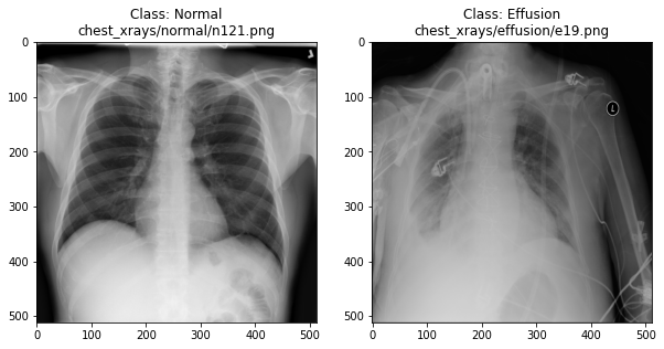

Can we detect effusion?

Run the following code to flip a coin to select an x-ray from our collection.

print("Effusion or not?")

# flip a coin
coin_flip = random.choice(["Effusion", "Normal"])
if coin_flip == "Normal":
    fn = random.choice(normal_list)
else:
    fn = random.choice(effusion_list)

# plot the image
image = cv2.imread(fn)
plt.imshow(image)

Show the answer:

# Jupyter doesn't allow us to print the image until the cell has run,
# so we'll print in a new cell.
print(f"The answer is: {coin_flip}!")

How does a computer see an image?

Consider an image as a matrix in which the value of each pixel corresponds to a number that determines a tone or color. Let’s load one of our images:

import numpy as np 

file_idx = 56
example = normal_list[file_idx]
image = cv2.imread(example)

print(image.shape)

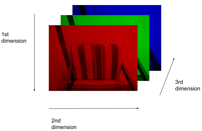
(512, 512, 3)

Here we see that the image has 3 dimensions. The first dimension is height (512 pixels) and the second is width (also 512 pixels). The presence of a third dimension indicates that we are looking at a color image (“RGB”, or Red, Green, Blue).

For more detail on image representation in Python, take a look at the Data Carpentry course on Image Processing with Python. The following image is reproduced from the section on Image Representation.

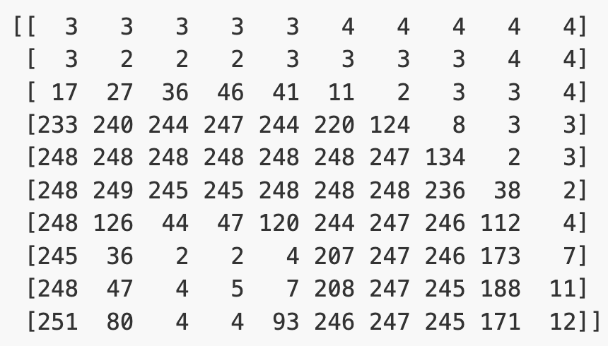
For simplicity, we’ll instead load the images in greyscale. A greyscale image has two dimensions: height and width. Greyscale images have only one channel. Most greyscale images are 8 bits per channel or 16 bits per channel. For a greyscale image with 8 bits per channel, each value in the matrix represents a tone between black (0) and white (255).

image = cv2.imread(example, cv2.IMREAD_GRAYSCALE)
print(image.shape)

(512, 512)

Let’s briefly display the matrix of values, and then see how these same values are rendered as an image.

# Print a 10 by 10 chunk of the matrix
print(image[35:45, 30:40])

# Plot the same chunk as an image
plt.imshow(image[35:45, 30:40], cmap='gray', vmin=0, vmax=255)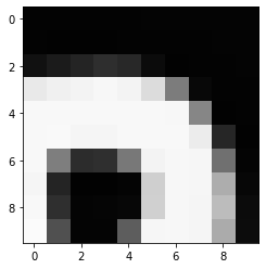

Image pre-processing

In the next section, we’ll be building and training a model. Let’s prepare our data for the modelling phase. For convenience, we’ll begin by loading all of the images and corresponding labels and assigning them to a list.

# create a list of effusion images and labels
dataset_effusion = [cv2.imread(fn, cv2.IMREAD_GRAYSCALE) for fn in effusion_list]
label_effusion = np.ones(len(dataset_effusion))

# create a list of normal images and labels
dataset_normal = [cv2.imread(fn, cv2.IMREAD_GRAYSCALE) for fn in normal_list]
label_normal = np.zeros(len(dataset_normal))

# Combine the lists
dataset = dataset_effusion + dataset_normal
labels = np.concatenate([label_effusion, label_normal])

# Downsample the images from (512,512) to (256,256)
dataset = [cv2.resize(img, (256,256)) for img in dataset]

# Check the size of the reshaped images
print(dataset[0].shape)

(256, 256)

# Standardize the data
# For each image: subtract the mean and divide by the standard deviation
for i in range(len(dataset)):
  dataset[i] = (dataset[i] - np.mean(dataset[i])) / np.std(dataset[i])

Reshaping

Finally, we’ll convert our dataset from a list to an array. We are expecting it to be (700, 256, 256), representing 700 images (350 effusion and 350 normal), each with dimensions 256×256.

PYTHON

dataset = np.asarray(dataset, dtype=np.float32)
print(f"Matrix Dimensions: {dataset.shape}")

OUTPUT

(700, 256, 256)

Exercise

Pick any grayscale image from your dataset (hint: dataset[idx]) and inspect the following:

1. What is the new shape of the image array?
   
2. What are the mean and standard deviation of the pixel values?

Show me the solution

1. Shape after resizing: dataset[0].shape (256, 256)
2. The mean is 0 (dataset[0].mean()) and the standard deviation is 1 (dataset[0].std())

We could plot the images by indexing them on dataset, e.g., we can plot the first image in the dataset with:

PYTHON

idx = 0
vals = dataset[idx].flatten()
plt.imshow(dataset[idx], cmap='gray', vmin=min(vals), vmax=max(vals))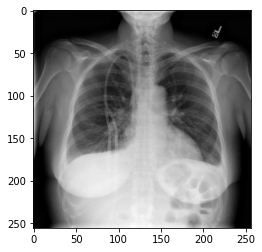

Key Points

• X-ray images can be loaded and visualized using Python libraries like OpenCV and NumPy.
• Images are stored as 2D arrays (grayscale) or 3D arrays (RGB).
• Visual inspection helps us understand how disease features appear in imaging data.
• Preprocessing steps like resizing and standardization prepare data for machine learning.