Image 1 of 1: ‘Dendrogram showing hierarchical clustering of tissue gene expression data.’
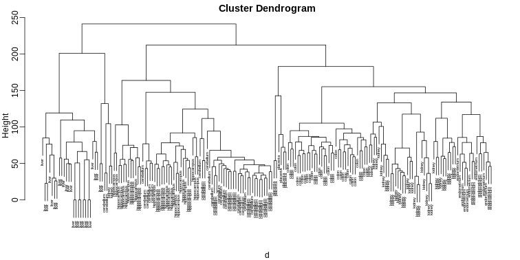
Dendrogram showing hierarchical clustering of tissue gene expression
data.
Figure 2
Image 1 of 1: ‘Dendrogram showing hierarchical clustering of tissue gene expression data with colors denoting tissues.’
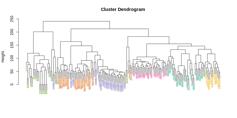
Dendrogram showing hierarchical clustering of tissue gene expression
data with colors denoting tissues.
Figure 3
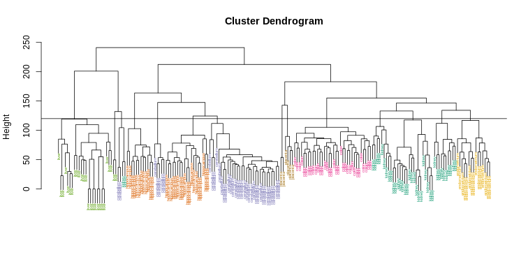
Image 1 of 1: ‘Dendrogram showing hierarchical clustering of tissue gene expression data with colors denoting tissues. Horizontal line defines actual clusters.’
Dendrogram showing hierarchical clustering of tissue gene expression
data with colors denoting tissues. Horizontal line defines actual
clusters.
Figure 4
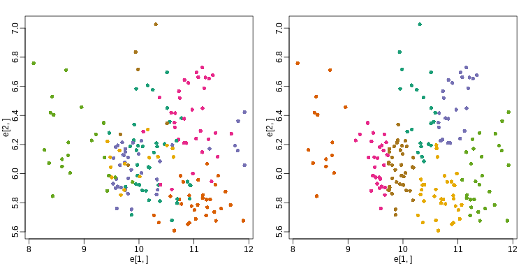
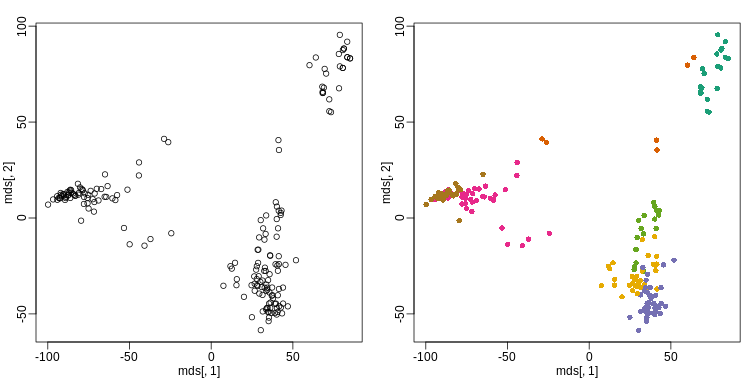
Image 1 of 1: ‘Plot of gene expression for first two genes (order of appearance in data) with color representing tissue (left) and clusters found with kmeans (right).’
Plot of gene expression for first two genes (order of appearance in
data) with color representing tissue (left) and clusters found with
kmeans (right).
Figure 5
Image 1 of 1: ‘Plot of gene expression for first two PCs with color representing tissues (left) and clusters found using all genes (right).’
Plot of gene expression for first two PCs with color representing
tissues (left) and clusters found using all genes (right).
Figure 6
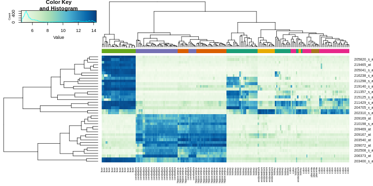
Image 1 of 1: ‘Heatmap created using the 40 most variable genes and the function heatmap.2.’
Heatmap created using the 40 most variable genes and the function
heatmap.2.
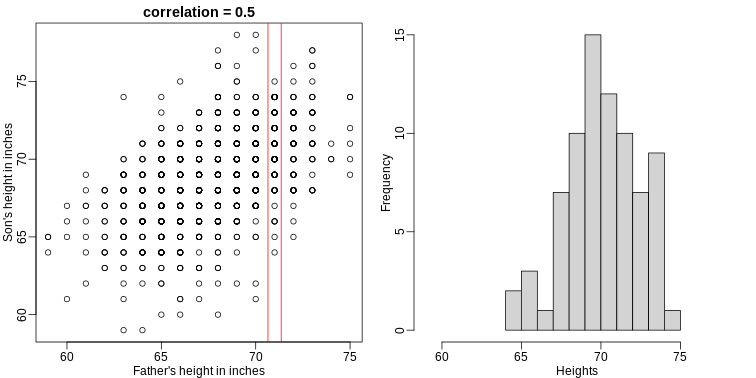
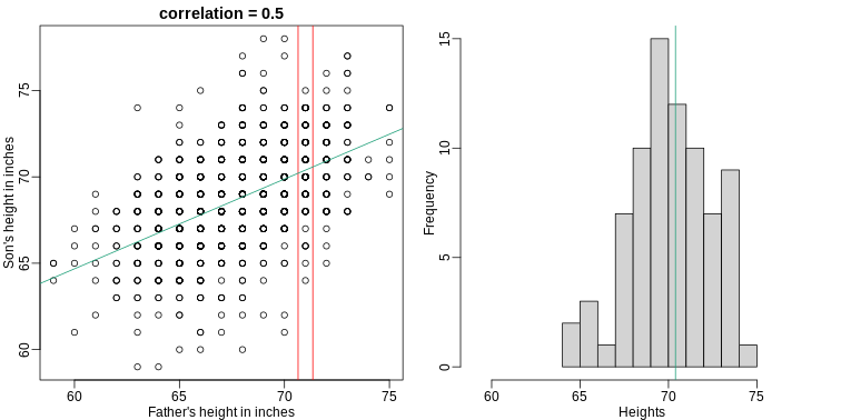
Image 1 of 1: ‘Son versus father height (left) with the red lines denoting the stratum defined by conditioning on fathers being 71 inches tall. Conditional distribution: son height distribution of stratum defined by 71 inch fathers.’
Son versus father height (left) with the red lines denoting the stratum
defined by conditioning on fathers being 71 inches tall. Conditional
distribution: son height distribution of stratum defined by 71 inch
fathers.
Figure 3
Image 1 of 1: ‘Son versus father height showing predicted heights based on regression line (left). Conditional distribution with vertical line representing regression prediction.’
Son versus father height showing predicted heights based on regression
line (left). Conditional distribution with vertical line representing
regression prediction.
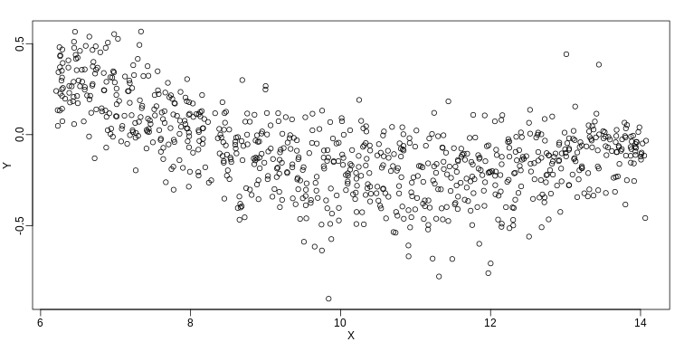
Image 1 of 1: ‘MA-plot comparing gene expression from two arrays.’
MA-plot comparing gene expression from two arrays.
Figure 2
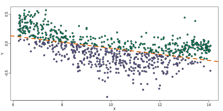
Image 1 of 1: ‘MA-plot comparing gene expression from two arrays with fitted regression line. The two colors represent positive and negative residuals.’
MA-plot comparing gene expression from two arrays with fitted regression
line. The two colors represent positive and negative residuals.
Figure 3
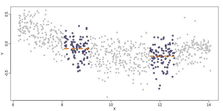
Image 1 of 1: ‘MAplot comparing gene expression from two arrays with bin smoother fit shown for two points.’
MAplot comparing gene expression from two arrays with bin smoother fit
shown for two points.
Figure 4
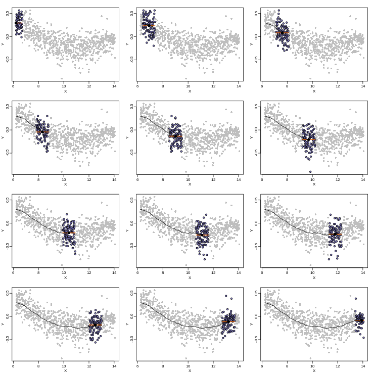
Image 1 of 1: ‘Illustration of how bin smoothing estimates a curve. Showing 12 steps of process.’
Illustration of how bin smoothing estimates a curve. Showing 12 steps of
process.
Figure 5
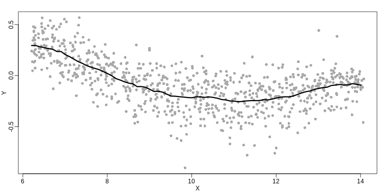
Image 1 of 1: ‘MA-plot with curve obtained with bin-smoothed curve shown.’
MA-plot with curve obtained with bin-smoothed curve shown.
Figure 6
Image 1 of 1: ‘MA-plot comparing gene expression from two arrays with bin local regression fit shown for two points.’
MA-plot comparing gene expression from two arrays with bin local
regression fit shown for two points.
Figure 7
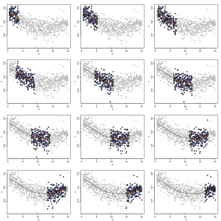
Image 1 of 1: ‘Illustration of how loess estimates a curve. Showing 12 steps of the process.’
Illustration of how loess estimates a curve. Showing 12 steps of the
process.
Figure 8
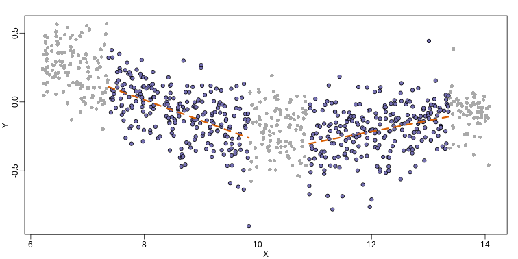
Image 1 of 1: ‘MA-plot with curve obtained with loess.’
MA-plot with curve obtained with loess.
Figure 9
Image 1 of 1: ‘Loess fitted with the loess function.’
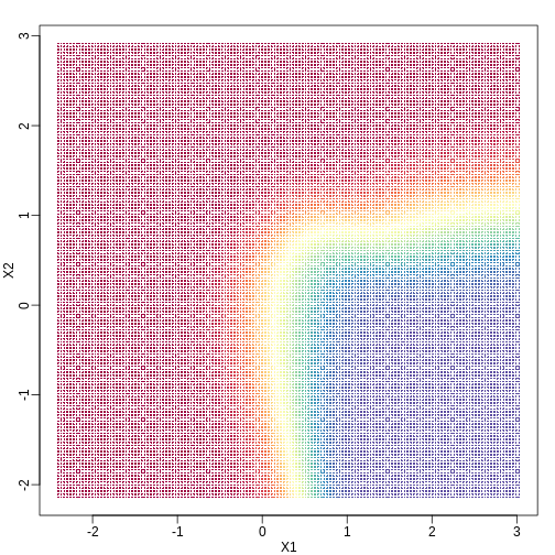
Image 1 of 1: ‘Probability of Y=1 as a function of X1 and X2. Red is close to 1, yellow close to 0.5, and blue close to 0.’
Probability of Y=1 as a function of X1 and X2. Red is close to 1, yellow
close to 0.5, and blue close to 0.
Figure 2
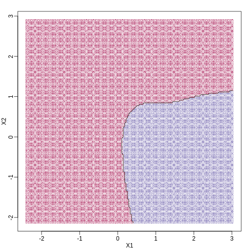
Image 1 of 1: ‘Bayes rule. The line divides part of the space for which probability is larger than 0.5 (red) and lower than 0.5 (blue).’
Bayes rule. The line divides part of the space for which probability is
larger than 0.5 (red) and lower than 0.5 (blue).
Figure 3
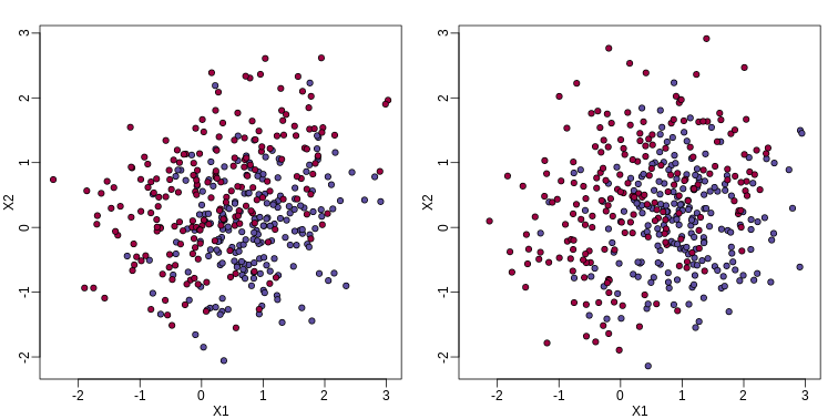
Image 1 of 1: ‘Training data (left) and test data (right).’
Training data (left) and test data (right).
Figure 4
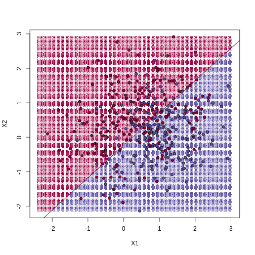
Image 1 of 1: ‘We estimate the probability of 1 with a linear regression model with X1 and X2 as predictors. The resulting prediction map is divided into parts that are larger than 0.5 (red) and lower than 0.5 (blue).’
We estimate the probability of 1 with a linear regression model with X1
and X2 as predictors. The resulting prediction map is divided into parts
that are larger than 0.5 (red) and lower than 0.5 (blue).
Figure 5
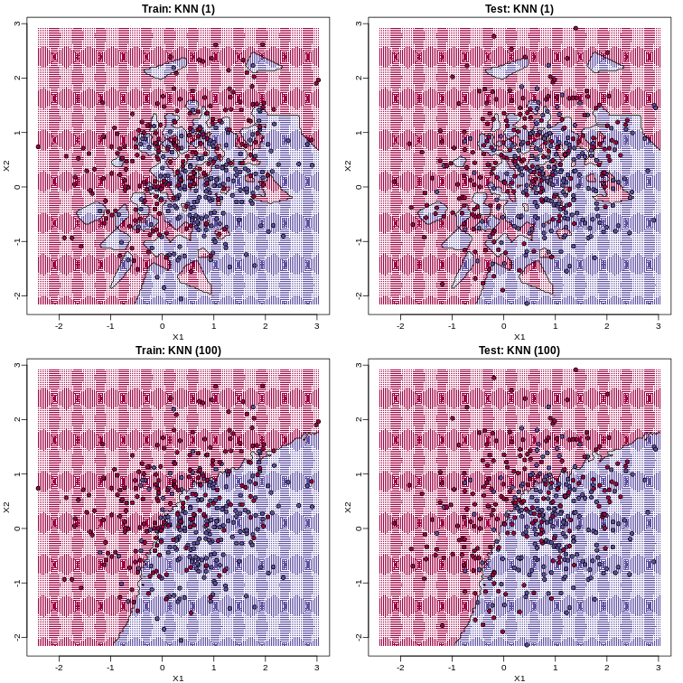
Image 1 of 1: ‘Prediction regions obtained with kNN for k=1 (top) and k=200 (bottom). We show both train (left) and test data (right).’
Prediction regions obtained with kNN for k=1 (top) and k=200 (bottom).
We show both train (left) and test data (right).
Figure 6
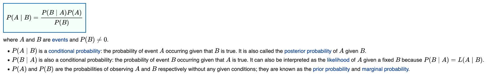
Image 1 of 1: ‘Bayes Rule 101 - From Wikipedia’
Bayes Rule 101 - From Wikipedia
Figure 7
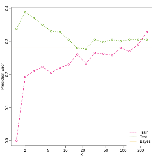
Image 1 of 1: ‘Prediction error in train (pink) and test (green) versus number of neighbors. The yellow line represents what one obtains with Bayes Rule.’
Prediction error in train (pink) and test (green) versus number of
neighbors. The yellow line represents what one obtains with Bayes Rule.
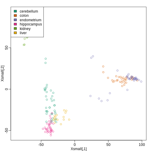
Image 1 of 1: ‘First two PCs of the tissue gene expression data with color representing tissue. We use these two PCs as our two predictors throughout.’
First two PCs of the tissue gene expression data with color representing
tissue. We use these two PCs as our two predictors throughout.
Figure 2
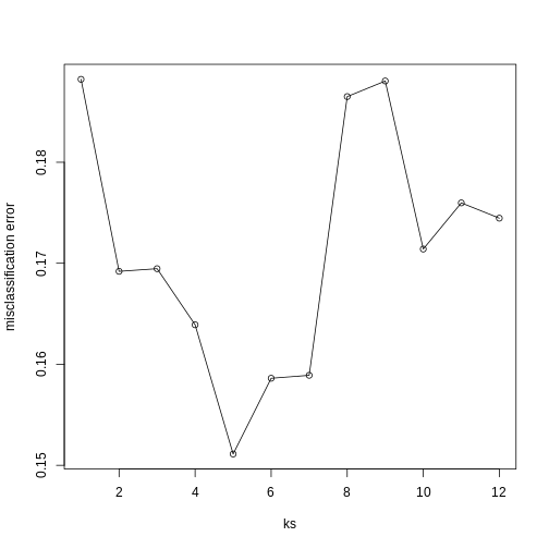
Image 1 of 1: ‘Misclassification error versus number of neighbors.’
Misclassification error versus number of neighbors.
Figure 3
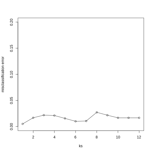
Image 1 of 1: ‘Misclassification error versus number of neighbors when we use 5 dimensions instead of 2.’
Misclassification error versus number of neighbors when we use 5
dimensions instead of 2.