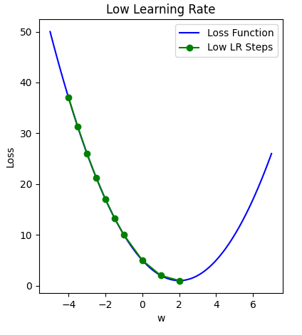
Image 1 of 1: ‘Plot of loss over weight value illustrating how a small learning rate takes a long time to reach the optimal solution.’
Small learning rate leads to inefficient
approach to loss minima
Figure 2
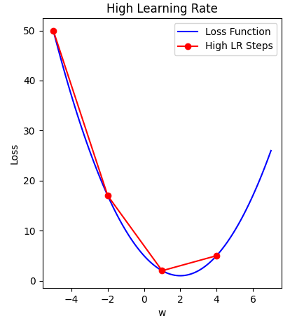
Image 1 of 1: ‘Plot of loss over weight value illustrating how a large learning rate never approaches the optimal solution because it bounces between the sides.’
A large learning rate results in overshooting
the gradient descent minima
Figure 3
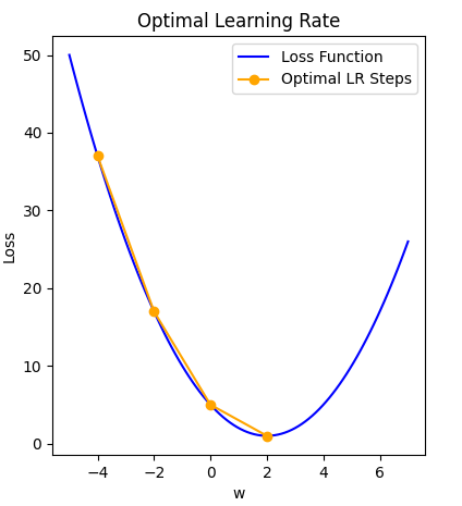
Image 1 of 1: ‘Plot of loss over weight value illustrating how a good learning rate gets to optimal solution gradually.’
An optimal learning rate supports a gradual
approach to the minima
Figure 4
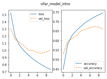
Image 1 of 1: ‘two panel figure; the figure on the left illustrates the training loss starting at 1.5 and decreasing to 0.7 and the validation loss decreasing from 1.3 to 1.0 before leveling out; the figure on the right illustrates the training accuracy increasing from 0.45 to 0.75 and the validation accuracy increasing from 0.53 to 0.65 before leveling off’
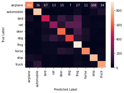
Image 1 of 1: ‘Confusion matrix of model predictions where the colour scale goes from black to light to represent values from 0 to the total number of test observations in our test set of 1000. The diagonal has much lighter colours, indicating our model is predicting well, but a few non-diagonal cells also have a lighter colour to indicate where the model is making a large number of prediction errors.’