
Scaling Study
Last updated on 2026-10-13 | Edit this page
Estimated time: 70 minutes
Overview
Questions
- How many resources should be requested for a given job?
- How does our application behave at different scales?
- Will the application benefit from requesting more computational resources?
Objectives
After completing this episode, participants should be able to …
- Perform a scaling study for a given application.
- Notice different perspectives on scaling parameters.
- Identify good working points for the job configuration.
Narrative:
- We panic, maybe we need more resources to meet the deadline with our title picture!
- Requesting resources with bigger systems requires a project proposal with an estimate of the resource demand
At times, you may think: “The deadline is approaching too fast and we may not finish our project in time.” Maybe requesting more resources from our clusters scheduler does the trick? How could we know if it helps and by how much?
Answering this question is often a formal requirement for compute time requests at larger HPC systems. They want to see good scaling behavior in an application, before they give access to a bigger chunk of their computational power. So, how well does your parallel application utilize larger number of resources? How well, does it scale?
What is Scaling?
The execution time of parallel applications changes with the number of parallel processes or threads. For example, when keeping the problem size fixed, i.e. keep the same amount of calculations, running the application with more processes/threads typically results in shorter execution times. We will consider the problem size as fixed for the first sections of this episode and discuss the case of a varying problem size later.
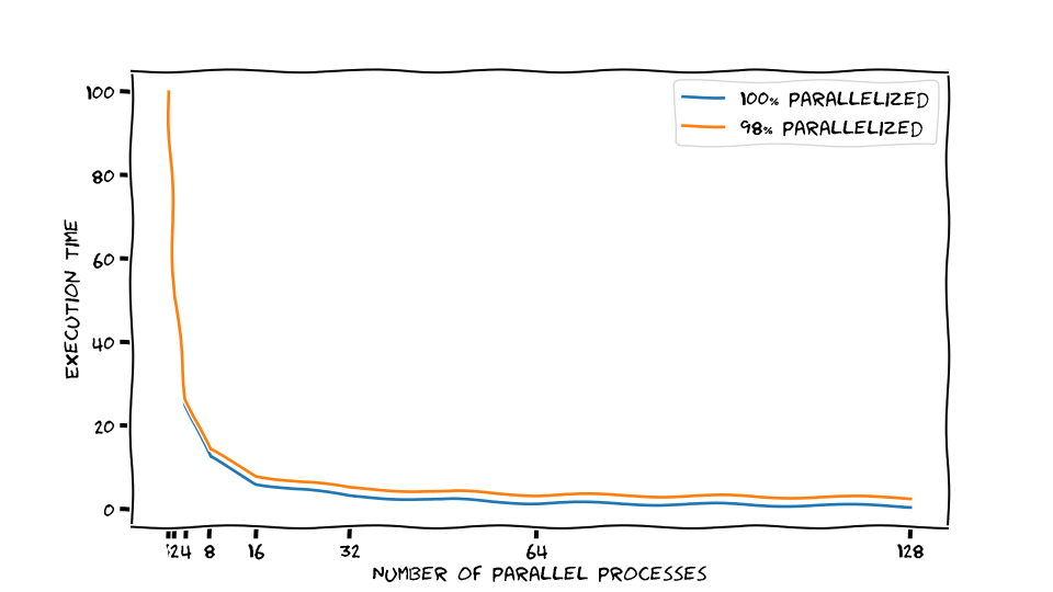
In a scaling study we measure how much a certain metric of an application, most commonly the execution time, changes with respect to the number of processes. In a common phrasing, this approach answers how the execution time scales with the number of parallel processors.
Starting from the job script render_snowman.sbatch:
We should address the various ways to start MPI programs at first use
and choose a single way. Preparing the software is also cluster-specific
(module load ...).
In the mid-/long-term this may call for a site-specific implementation of the course, e.g. via the hpc-intro workbench.
BASH
#!/usr/bin/bash
#SBATCH --time=01:00:00
#SBATCH --nodes=1
#SBATCH --mem-per-cpu=200MB

# The `module load` command you had to load for building the raytracer
module load 2025 GCC/13.2.0 OpenMPI/4.1.6 buildenv/default Boost/1.83.0 CMake/3.27.6 libpng/1.6.40

time mpirun -- ./raytracer -width=800 -height=800 -spp=128 -png "$(date +%Y-%m-%d_%H%M%S).png"
we can manually run such a scaling study by submitting multiple jobs.
In OpenMPI versions 4 and 5 the number of Slurm tasks is automatically
picked up, so we do not set -n or -np of
mpirun. We use -- to separate the arguments of
mpirun (none in this case) from the MPI application
raytracer and its arguments. Otherwise you may experience
errors in some versions of OpenMPI 5, where mpirun
misinterprets the arguments of raytracer as its own.
Scaling other resources with number of CPU cores
When scaling the resources outside of the job script, e.g. with
sbatch --ntasks=X ..., as done above, we make sure to scale
other resource requirements with the number of parallel processors. In
this case, --mem-per-cpu=200MB is necessary to scale the
amount of memory with the number of processors. --mem
requests a fixed amount of memory per node.
For example, if each MPI process needs \(100\,\)MB, requesting \(2\,\)GB would only be enough for up to 20 MPI processes.
Forgetting a limit like this is a common pitfall in this situation.
Let’s start some measurements with \(1\), \(2\), \(4\), and \(8\) tasks:
OUTPUT
$ sbatch --ntasks 1 render_snowman.sbatch
Submitted batch job 16142767
$ sbatch --ntasks 2 render_snowman.sbatch
Submitted batch job 16142768
$ sbatch --ntasks 4 render_snowman.sbatch
Submitted batch job 16142769
$ sbatch --ntasks 8 render_snowman.sbatch
Submitted batch job 16142770
Now we have to wait until all four jobs are finished.
Regular update of squeue
You can use squeue --me -i 30 to get an update of all of
your jobs every 30 seconds.
If you don’t need a more regular update, it is good practice to keep the interval on the order of 30s to a couple of minutes, just to be nice to Slurms server resources.
Once the jobs are finished, we can use
grep "real" slurm-*.out to get the wall clock time of all
four jobs:
OUTPUT
slurm-16142767.out:real       2m7.218s
slurm-16142768.out:real       1m7.443s
slurm-16142769.out:real       0m32.584s
slurm-16142770.out:real       0m17.480s
The real-time is decreasing significantly each time we
double the number of Slurm tasks. From this, we feel that doubling the
number of CPU cores really is a winning strategy!
Exercise: Continue scaling study to larger values
Run the same scaling study and continue it for even larger number of
--ntasks, e.g. 16, 32, 64, 128. So far, we have been using
--nodes=1 to stay on a single node. At which point are your
MPI processes distributed across more than one node? Use Slurm command
line tools to find out the how many CPU cores (MPI processes) are
available on a single node. You may have to increase the number of nodes
with --nodes, if you want to go beyond that limit.
Gather your real time results and place them in a
.csv file. Here is an example for our previous
measurements:
ntasks,time
1,127.218
2,67.443
4,32.584
8,17.480
...
How much does each doubling of the CPU resources help with running the parallel raytracer?
You can use sinfo to find out the node names of your
particular Slurm partition. Then use scontrol to show all
details about a single node from that partition. It will show you the
number of CPU (cores) available on that node.
ntasks,time
1,127.218
2,67.443
4,32.584
8,17.480
16,10.251
32,7.257
64,8.044
128,8.575
Using grep "real" slurm-*.out, we can see the execution
time is halved in the beginning, with each doubling of the CPU cores.
However, somewhere between \(8\) and
\(16\) cores, we start to see less and
less improvement.
Adding more resources does not help indefinitely. At some point the overhead of managing the calculation in separate tasks outweighs the benefit of parallel calculation. There is too little to do in each tasks and the overhead starts to dominate.
At some point adding more CPU cores does not help us anymore.
info dump below in this section
Maybe be more specific about which overheads and how we can see them?
Adding more CPU cores can actively slow down the calculation after a certain point. The optimal point is different for each application and each configuration. It depends on the ratio between calculations, communications and various management overheads in the whole process of running everything.
Overheads and Reliable Measurements
Many overheads and when they show also depend on the underlying hardware. So the sweet spot may very well be different for different clusters, even if the application and configuration stays the same! For example, network communication always introduces latencies (short waiting times) for each connection and their bandwidth determines how long a communication takes. Here, clusters using different network architectures and technologies often exhibit different scaling behavior and configuration sweet spots for your applications.
Another common issue lies within our measurements themself. We
perform a single time measurement on a worker node that is possibly
shared with other jobs at the same time. What if another user runs an
application that hogs shared resources like the local disk or network
interface card? In this case our measurements become somewhat
non-deterministic. Running the same measurement twice may result in
significantly different values. If you need reliable results, e.g. for a
publication, requesting exclusive access to Slurms resources through the
sbatch flag --exclusive is the best approach.
As a drawback, this typically results in longer waiting times, since
whole nodes have to be reserved for the measurement jobs, even if not
all resources are used.
Even on exclusive resources, the measurements cannot be 100% reliable. For example, the scheduling behavior of the Linux kernel, or access to remote resources like the parallel file system or data from the web, are still affecting your measurements in unpredictable ways. Therefore, the best results are achieved by taking the mean and standard deviations of repeated measurements for the same configuration. The measured minimum also has strong informative value, since it proofs the best observed behavior.
Keep in mind, --exclusive will always request all
resources of a given node, even if only few cores are used. In these
cases, tools like seff show worse resource utilization
results, since measurements are done with respect to all booked
resources.
Scaling studies can also be done with respect to different application and job parameters. For example, what is the execution time when we change the workload, e.g. a larger number of pixels, samples per pixels, or a more complex scene? How much does a communication overhead change, if we change the number of involved nodes while keeping the workload and number of tasks fixed, i.e. changing the network communication surface? Scaling studies like these can help identify pressure points that affect the applications performance.
Scaling studies typically occur in a preparation phase where the application is evaluated with a representative example workload. Once a good configuration is found, we know the application is running close to an optimal performance and larger number of calculations can start, often called the production phase.
In a similar vein, scaling studies can be a formal requirement for compute time applications on larger HPC systems. On these systems and for larger calculation campaigns it is more crucial to run efficient calculations, since the resources are typically more contested and the potential energy- and carbon footprint becomes much larger.
Speedup, Efficiency, and Strong Scaling
To quantitatively and empirically study the scaling behavior of a given application, it is common to look at the speedup and efficiency with respect to adding more parallel processors.
Speedup is a metric to compare the execution times with different amounts of resources. It answers the question
How much faster is the application with \(N\) parallel processes/threads, compared to the serial execution with \(1\) process/thread)?
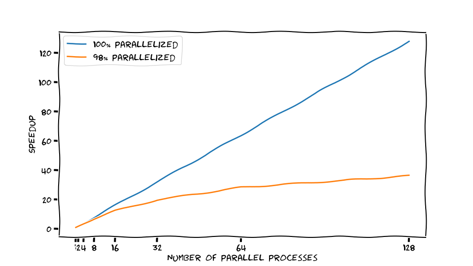
Speedup is defined by the comparison of wall times \(T(N)\) of the application with \(N\) parallel processes: \[S(N) = \frac{T(1)}{T(N)}\] Here, \(T(1)\) is the wall time for a sequential execution, and \(T(N)\) is the execution with \(N\) parallel processes. For our raytracer, with \(2\) processes, we observe a speedup of \(S(2) = \frac{127.218}{67.443} \approx 1.89\) In reality, our application only got \(1.89\times\) faster, for the \(2\) parallel processes we have spent on it. Ideally, we would have expected a speedup of \(2\), so our application does not seem perfectly efficient in terms of using the additional parallel processes to be faster.
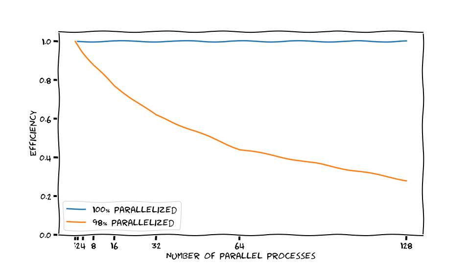
We can calculate the efficiency with wich each additional parallel process contributes to the applications speedup: \[\eta(N) = \frac{S(N)}{N}\]
Exercise: Calculate Speedup and Efficency
Extend the .csv file of your measurements from above
with a speedup and efficiency column. It may
look like this:
ntasks,time,speedup,efficiency
1,127.218,1.00,1.00
2,67.443,1.89,0.94
4,32.584,3.90,0.98
8,17.480,7.28,0.91
...
You may want to use any data visualization tool, e.g. python or spreadsheets, to visualize the data.
What number of processes may be a good working point for the raytracer with \(800 \times 800\) pixel and \(128\) samples per pixel?
For all of our measurements, the speedup and efficiencies are
ntasks,time,speedup,efficiency
1,127.218,1.00,1.00
2,67.443,1.89,0.94
4,32.584,3.90,0.98
8,17.480,7.28,0.91
16,10.251,12.41,0.78
32,7.257,17.53,0.55
64,8.044,15.82,0.25
128,8.575,14.84,0.12
Plotting the speedup and efficiency helps with identifying a good working point:
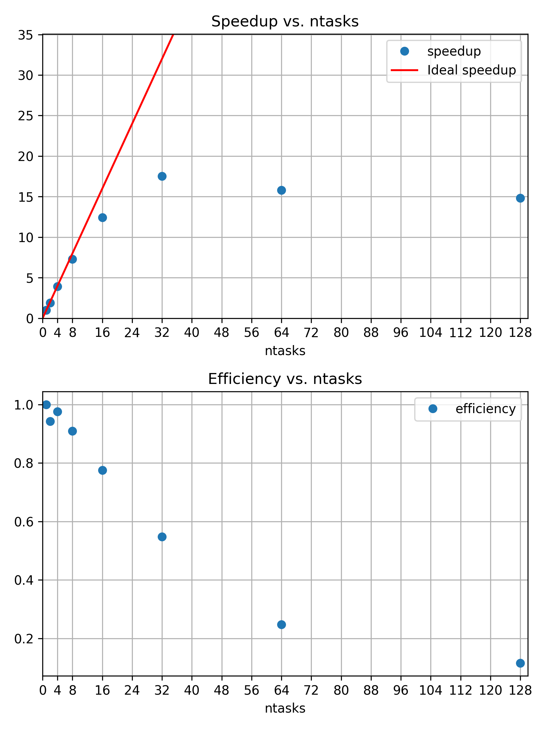
The 16th processor is still close to 80% efficient. The corresponding speedup is less than the theoretical optimum, which is visualized by a red line of slope \(1\).
There is no exact optimum and the best working point is open for discussion. However, it would be difficult to justify additional cores, if their contribution to speedup is only 50% efficient or even less.
Discussion: Why does the Speedup Efficiency drop?
Adding more and more resources is not always speeding up our application. What may be possible reasons for worse speedup efficiency at larger numbers of parallel processors/threads?
Briefly collect and discuss any reasons you can think of.
If you have experience with python, you can use our python script to create the
same plots as above, but for your own data. It depends on
numpy, pandas, and matplotlib, so
make sure to prepare a corresponding python environment.
The script expects your .csv files to be called
strong.csv and weak.csv, and be placed in the
same directory.
So far, we kept the workload size fixed to \(800 \times 800\) pixels and \(128\) samples per pixel for the same scene with three snowman. The diminishing returns for adding more and more parallel processors leads to a famous observation. The speedup of a program through parallelization is limited by the execution time of the serial fraction that is not parallelizable. No application is 100% parallelizable, so adding an arbitrary amount of parallel processors can only affect the parallelizable section. In the best case, the execution time gets reduced to the serial fraction of the application.
An application is said to scale strongly, if adding more cores significantly reduces the execution time.
Amdahls Law1
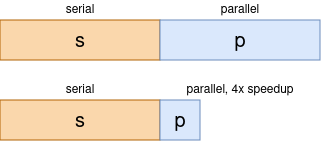
The speedup of a program through parallelization is limited by the execution time of the serial fraction that is not parallelizable. For a given execution time \(T(N) = s + \frac{p}{N}\), with \(s\) the serial fraction, and \(p\), the parallel fraction of the applications execution time, speedup \(S\) is defined as \[S(N) = \frac{T(1)}{T(N)} = \frac{1}{s + \frac{p}{N}} \Rightarrow \lim_{N\rightarrow \infty} S(N) = \frac{1}{s}\]
In other words, increasing the number of parallel processes \(N\) for an application that only has a serial part that is taking up \(1\)% of the execution time, will never exceed a speedup of \(\frac{1}{s} = \frac{1}{0.01} = 100\). No matter how many processes we will use!
Discussion: When should we stop adding CPU cores?
Discuss your previous results and decide on a good working point. How many cores are still usefully reducing the execution time.
What other factors could affect your decision, e.g. available hardware and corresponding waiting times.
The learners should realize there is a point of diminishing returns. Where exactly to draw the line is debatable, but in the previous example \(N=32\) seems to be a sweet spot with the best Speedup and an efficiency \(>50\)%.
There are many reasons why a large number of parallel processes may result in worse speedup. Among others, it may be due to I/O overhead, synchronization between threads, or a limited divisibility of the problem domain, where additional processors could not solve additional work.
If scaling is limited, why are there larger HPC systems? Weak scaling.
For a fixed problem size, we observed that adding more parallel processors can only help up to a certain point. But what if the project benefits from increasing the workload size, i.e. doing more calculations? For example, does a higher resolution, more accuracy, or more statistics, etc., improve our insights and results? In this case, our perspective on efficiency changes and we address a different optimization than before: Doing more calculations with an increasing number of parallel processors. For our raytracer example, increasing the workload corresponds to more pixels, more samples per pixel, and/or a more complex scene.
Weak scaling refers to the scaling behavior of an application for a fixed workload per parallel processing unit, e.g. increasing the number of pixels by the same amount as the number of parallel processors \(N\).
The difference between strong and weak scaling
In the previous discussion about Amdahls Law we kept the total amount of calculations fixed and increased the number of parallel processors \(N\). Now, we are transitioning to a different perspective where we increase both, the number total amount of calculations and the number of parallel processors \(N\),
In the former, we reach an absolute limit for moderate numbers of \(N\) and would not benefit from increasing the number of parallel processes \(N\). In the later case, we may benefit solving more calculations and we hope to be back in the business of Supercomputers with an \(N\) in the order of thousands!
To scale the workload of the snowman raytracer, we can increase the number of calculated pixels with the same factor with which we increase the number of parallel processors. For one processor we have \(800 \times 800 = 640000\) pixel. That means for two processors we need a height and a width of \(\sqrt{2 \times 640000} = 1131.371 \approx 1131\). And similarly increasing the number of pixels for \(--ntasks=4\) and so on.
The job script could look like this:
BASH
#!/usr/bin/bash
#SBATCH --time=01:00:00
#SBATCH --nodes=1
#SBATCH --mem-per-cpu=3800MB

module load 2025 GCC/13.2.0 OpenMPI/4.1.6 buildenv/default Boost/1.83.0 CMake/3.27.6 libpng/1.6.40

# Create associative array
declare -A pixel
pixel[1]="800"
pixel[2]="1131"
pixel[4]="1600"
pixel[8]="2263"
pixel[16]="3200"
pixel[32]="4526"
pixel[64]="6400"

time mpirun -- ./build/raytracer -width=${pixel[${SLURM_NTASKS}]} -height=${pixel[${SLURM_NTASKS}]} -spp=128 -threads=1 -png "$(date +%Y-%m-%d_%H%M%S).png"In each scaling study, it is crucial to identify which application parameters affect the execution time. There are often multiple ways.
For the snowman raytracer, instead of changing the total number of
pixels, we can multiply the number of parallel MPI processes
(${SLURM_NTASKS}) with the samples per pixel (starting from
-spp=128). For a single process, the whole \(800 \times 800\) pixel picture is
calculated in a single MPI process with 128 per pixel. Running with two
MPI processes, both have to calculate half the number of pixels, but
twice the amount of samples per pixel.
BASH
#!/usr/bin/bash
#SBATCH --time=01:00:00
#SBATCH --nodes=1
#SBATCH --mem-per-cpu=500MB

module load 2025 GCC/13.2.0 OpenMPI/4.1.6 buildenv/default Boost/1.83.0 CMake/3.27.6 libpng/1.6.40

SPP="$[${SLURM_NTASKS}*128]"

time mpirun -- ./build/raytracer -width=800 -height=800 -spp=${SPP} -threads=1 -png "$(date +%Y-%m-%d_%H%M%S).png"

In direct comparison, and zooming in really close, you can see more noise in Figure 1, e.g. in the shadows, relative to Figure 2. One could argue that we passed the point of diminishing returns, though. Is a \(64\times\) increase in computational cost worth the observed quality improvement? For the samples per pixel, we seem to not benefit much from weak scaling. Larger resolutions, by increasing the number of pixels, may be a more useful dimension to increase in this case.
The usefulness of any computation can only be determined in the context of your scientific goals.
Increasing the resolution may be worth the effort, if we have a use for a larger, more detailed picture. In practice, there is a cutoff, beyond which no reasonable improvement is to be expected. This is a question about accuracy, error margins, and overall quality, which can only be answered in the specific context of each research project. If there is no tangible benefit of increasing the workload, running at a larger number of parallel processes does not serve a purpose, even if the application still exhibits good “weak scaling efficiency”.
If we increase the workload at the rate as our number of parallel processes (\(N\)) our speedup is defined as \[S_{\text{weak}}(N) = \frac{T(1)}{T(N)} \times N\] since we do \(N\) times more work with \(N\) processors, compared to our reference \(T(N=1)\). Efficiency is still defined as \[\eta_{\text{weak}}(N) = \frac{S_{\text{weak}}(N)}{N} = \frac{T(1)}{T(N)}\]
Exercise: Weak scaling
Repeat the previous scaling study and increase the number of pixels accordingly to study the raytracers weak scaling behavior.
- Run with 1, 2, 4, 8, 16, 32, 64 MPI processes on single node
- Take
timemeasurements and consider running with--exclusiveto ensure more reliable results. - Create a
.csvfile and run the plotting script
ntasks, pixel,    time, speedup, efficiency
     1,   800, 123.162,     ???,        ???
     2,  1131, 122.562,     ???,        ???
     4,  1600,     ???,     ???,        ???
     8,  2263,     ???,     ???,        ???
...
How well does the application scale with an increasing workload size?
Do you see a qualitative difference in the resulting .png
files and is the increased sample-per-pixel size worth the computational
costs?
ntasks, pixel,    time, speedup, efficiency
     1,   800, 123.162,    1.00,       1.00
     2,  1131, 122.562,    2.01,       1.00
     4,  1600, 124.522,    3.96,       0.99
     8,  2263, 125.606,    7.84,       0.98
    16,  3200, 125.803,   15.66,       0.98
    32,  4526, 130.137,   30.28,       0.95
    64,  6400, 138.636,   56.86,       0.89
The scaling behavior is reaching an asymptotic limit, where each additional processor is contributing with the same efficiency to the increased workload.
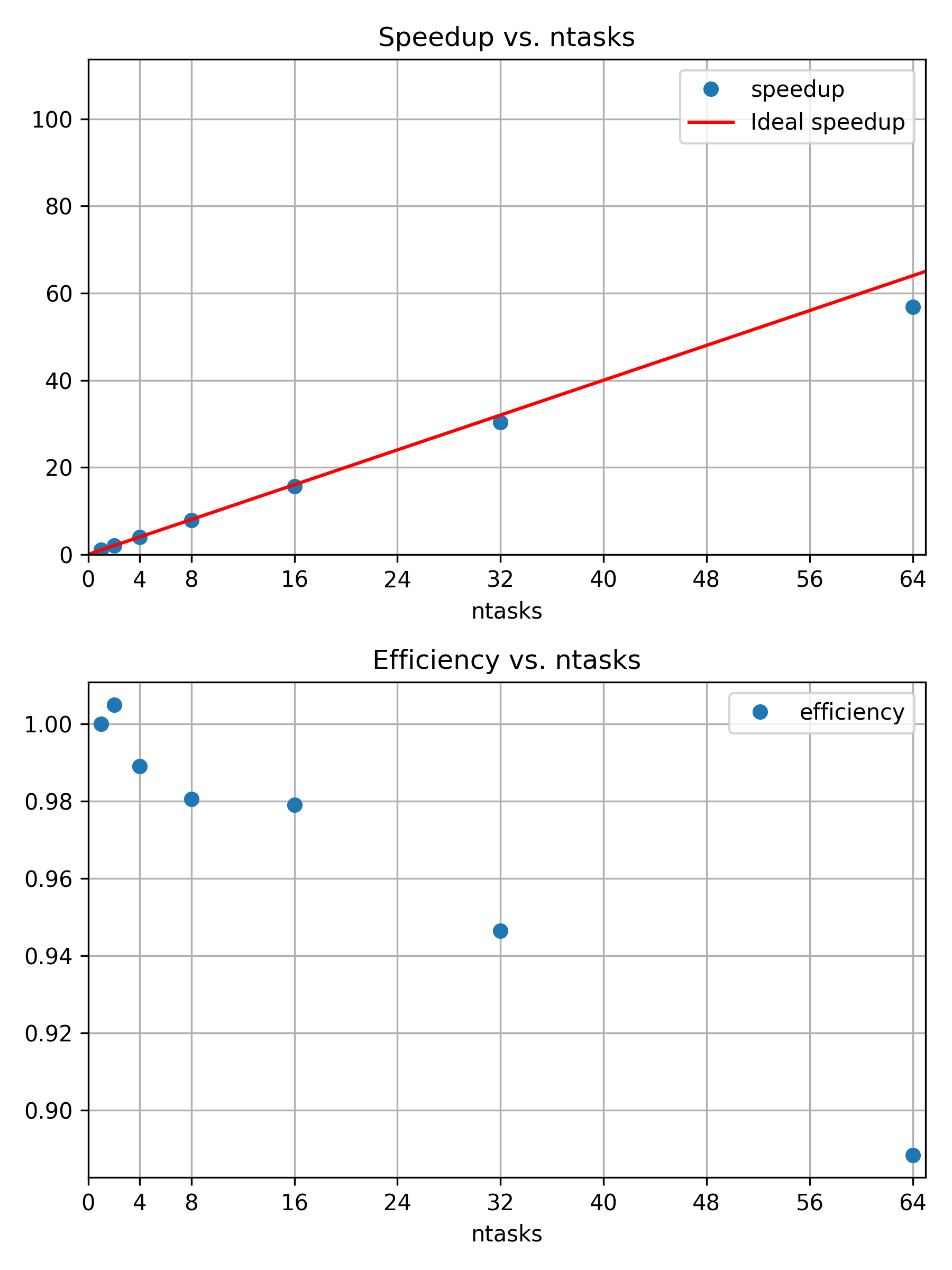
Weakly scaling jobs can make efficient use of a huge amount of resources.
The most important question is, if an increased workload is producing useful results. Here, we have the rendered picture of three snowmen in 800x800 with 128 samples per pixel and three snowmen in 6400x6400 with 128 samples per pixel. The second image has a much higher resolution. However, going way beyond \(6400 \times 6400\) pixels is probably not very meaningful, unless you are trying to print the worlds largest ad boards or similar.


Gustafsons Law2
A program scales on \(N\) parallel processors, if the problem size also scales with the number of processors. The speedup \(S\) becomes \[\text{S(N)} = \frac{s+pN}{s+p} = s+pN = s+(1-s)N\] with \(N\) processors, \(s\) the serial fraction, and \(p\) the parallel fraction of the execution time.
Summary
In this episode, we have seen that we can study the scaling behavior of our application with respect to different metrics, while varying its configuration. Most commonly, we study the execution time of an application with an increasing number of parallel processors. In such a scaling study, we collect comparable walltime measurements for an increasing number of Slurm tasks of a parallelizable and representative job. If a good working point is found, larger scale “production” jobs can be submitted to the HPC system.
If the application has good strong scaling behavior, adding more cores leads to an effective improvement in execution time. We observe diminishing returns of adding more cores to a fixed-size problem, so there is a (subjective) optimal number of parallel processors for a given application configuration. (Amdahls Law)
If increasing the workload size leads to better results, maybe because of improved accuracy and quality, we can study the weak scaling behavior and increase the workload size by the same factor of increasing parallel processors.
A good working point depends on the availability of resources, specifics of the underlying hardware, the particular application, and a particular configuration for the application. For that reason, scaling studies are a common requirement for formal compute time applications to prove an efficient execution of a given application.
We can study the impact of any parameter on metrics like, for example, walltime, CPU utilization, FLOPS, memory utilization, communication, output size on disk, and so on.
If you find yourself repeating similar measurements over and over again, you may be interested in an automation approach. This can be done by creating reproducible HPC workflows using JUBE, among other things.
Up to now, we were still working with basic metrics like the wall-clock time. In the next episode, we start with more in-depth measurements of many other aspects of our job and application.
- Jobs behave differently with increasing parallel resources and fixed or scaling workloads
- Scaling studies can help to quantitatively grasp this changing behavior
- Good working points are defined by configurations where more cores still provide sufficient speedup or improve quality through increasing workloads
- Amdahl’s law: speedup is limited by the serial fraction of a program
- Gustafson’s law: more resources for parallel processing still help, if larger workloads can meaningfully contribute to project results
G. M. Amdahl, ‘Validity of the single processor approach to achieving large scale computing capabilities’, in Proceedings of the April 18-20, 1967, spring joint computer conference, in AFIPS ’67 (Spring). New York, NY, USA: Association for Computing Machinery, Apr. 1967, pp. 483–485. doi: 10.1145/1465482.1465560.↩︎
J. L. Gustafson, ‘Reevaluating Amdahl’s law’, Commun. ACM, vol. 31, no. 5, pp. 532–533, May 1988, doi: 10.1145/42411.42415.↩︎