Vector data in Python
Last updated on 2023-08-14 | Edit this page
Overview
Questions
- How can I read, inspect, and process spatial objects, such as points, lines, and polygons?
Objectives
- Load spatial objects.
- Select the spatial objects within a bounding box.
- Perform a CRS conversion of spatial objects.
- Select features of spatial objects.
- Match objects in two datasets based on their spatial relationships.
Introduction
As discussed in Episode 2: Introduction to Vector Data, vector data represents specific features on the Earth’s surface using points, lines, and polygons. These geographic elements can then have one or more attributes assigned to them, such as ‘name’ and ‘population’ for a city, or crop type for a field. Vector data can be much smaller in (file) size than raster data, while being very rich in terms of the information captured.
In this episode, we will be moving from working with raster data to
working with vector data. We will use Python to open and plot point,
line, and polygon vector data. In particular, we will make use of the geopandas
package to open, manipulate and write vector datasets.
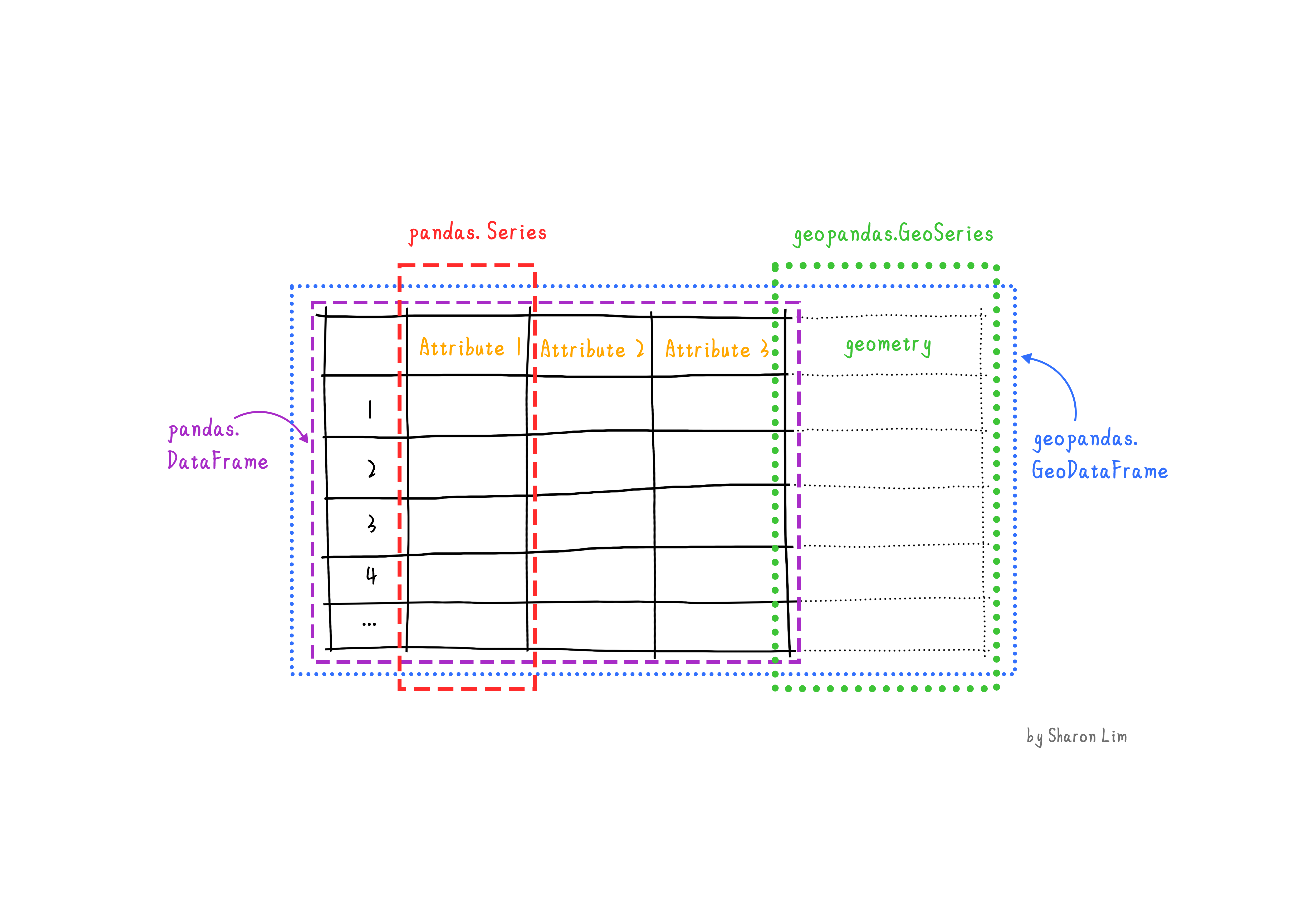
geopandas extends the popular pandas
library for data analysis to geospatial applications. The main
pandas objects (the Series and the
DataFrame) are expanded to geopandas objects
(GeoSeries and GeoDataFrame). This extension
is implemented by including geometric types, represented in Python using
the shapely library, and by providing dedicated methods for
spatial operations (union, intersection, etc.). The relationship between
Series, DataFrame, GeoSeries and
GeoDataFrame can be briefly explained as follow:
- A
Seriesis a one-dimensional array with axis, holding any data type (integers, strings, floating-point numbers, Python objects, etc.) - A
DataFrameis a two-dimensional labeled data structure with columns of potentially different types1. - A
GeoSeriesis aSeriesobject designed to store shapely geometry objects. - A
GeoDataFrameis an extenedpandas.DataFrame, which has a column with geometry objects, and this column is aGeoSeries.
In later episodes, we will learn how to work with raster and vector data together and combine them into a single plot.
Introduce the Vector Data
In this episode, we will use the downloaded vector data in the
data directory. Please refer to the setup page on how to download the data.
Import Vector Datasets
We will use the geopandas package to load the crop field
vector data we downloaded at:
data/brpgewaspercelen_definitief_2020_small.gpkg.
The data are read into the variable fields as a
GeoDataFrame. This is an extened data format of
pandas.DataFrame, with an extra column
geometry.
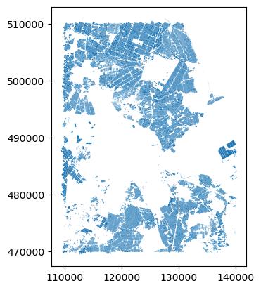
This file contains a relatively large number of crop field parcels. Directly loading a large file to memory can be slow. If the Area of Interest (AoI) is small, we can define a bounding box of the AoI, and only read the data within the extent of the bounding box.
PYTHON
# Define bounding box
xmin, xmax = (110_000, 140_000)
ymin, ymax = (470_000, 510_000)
bbox = (xmin, ymin, xmax, ymax)
Using the bbox input argument, we can load only the
spatial features intersecting the provided bounding box.
PYTHON
# Partially load data within the bounding box
fields = gpd.read_file("data/brpgewaspercelen_definitief_2020_small.gpkg", bbox=bbox)
How should I define my bounding box?
For simplicity, here we assume the Coordinate Reference System (CRS) and extent of the vector file are known (for instance they are provided in the dataset documentation).
You can also define your bounding box with online coordinates visualization tools. For example, we can use the “Draw Rectangular Polygon” tool in geojson.io.
Some Python tools, e.g. fiona(which
is also the backend of geopandas), provide the file
inspection functionality without the need to read the full data set into
memory. An example can be found in the
documentation of fiona.
And we can plot the overview by:
Vector Metadata & Attributes
When we read the vector dataset with Python (as our
fields variable) it is loaded as a
GeoDataFrame object. The read_file() function
also automatically stores geospatial information about the data. We are
particularly interested in describing the format, CRS, extent, and other
components of the vector data, and the attributes which describe
properties associated with each vector object.
We will explore
- Object Type: the class of the imported object.
- Coordinate Reference System (CRS): the projection of the data.
- Extent: the spatial extent (i.e. geographic area that the data covers). Note that the spatial extent for a vector dataset represents the combined extent for all spatial objects in the dataset.
Each GeoDataFrame has a "geometry" column
that contains geometries. In the case of our fields object,
this geometry is represented by a shapely.geometry.Polygon
object. geopandas uses the shapely library to
represent polygons, lines, and points, so the types are inherited from
shapely.
We can view the metadata using the .crs,
.bounds and .type attributes. First, let’s
view the geometry type for our crop field dataset. To view the geometry
type, we use the pandas method .type on the
GeoDataFrame object, fields.
OUTPUT
0        Polygon
1        Polygon
2        Polygon
3        Polygon
4        Polygon
          ...
22026    Polygon
22027    Polygon
22028    Polygon
22029    Polygon
22030    Polygon
Length: 22031, dtype: object
To view the CRS metadata:
OUTPUT
<Derived Projected CRS: EPSG:28992>
Name: Amersfoort / RD New
Axis Info [cartesian]:
- X[east]: Easting (metre)
- Y[north]: Northing (metre)
Area of Use:
- name: Netherlands - onshore, including Waddenzee, Dutch Wadden Islands and 12-mile offshore coastal zone.
- bounds: (3.2, 50.75, 7.22, 53.7)
Coordinate Operation:
- name: RD New
- method: Oblique Stereographic
Datum: Amersfoort
- Ellipsoid: Bessel 1841
- Prime Meridian: Greenwich
Our data is in the CRS RD New. The CRS is critical
to interpreting the object’s extent values as it specifies units. To
find the extent of our dataset in the projected coordinates, we can use
the .total_bounds attribute:
OUTPUT
array([109222.03325 , 469461.512625, 140295.122125, 510939.997875])This array contains, in order, the values for minx, miny, maxx and maxy, for the overall dataset. The spatial extent of a GeoDataFrame represents the geographic “edge” or location that is the furthest north, south, east, and west. Thus, it represents the overall geographic coverage of the spatial object.
We can convert these coordinates to a bounding box or acquire the index of the Dataframe to access the geometry. Either of these polygons can be used to clip rasters (more on that later).
Further crop the dataset
We might realize that the loaded dataset is still too large. If we
want to refine our area of interest to an even smaller extent, without
reloading the data, we can use the cx
indexer:
Export data to file
We will save the cropped results to a shapefile (.shp)
and use it later. The to_file function can be used for
exportation:
This will write it to disk (in this case, in ‘shapefile’ format),
containing only the data from our cropped area. It can be read again at
a later time using the read_file() method we have been
using above. Note that this actually writes multiple files to disk
(fields_cropped.cpg, fields_cropped.dbf,
fields_cropped.prj, fields_cropped.shp,
fields_cropped.shx). All these files should ideally be
present in order to re-read the dataset later, although only the
.shp, .shx, and .dbf files are
mandatory (see the Introduction to
Vector Data lesson for more information.)
Selecting spatial features
From now on, we will take in a point dataset
brogmwvolledigeset.zip, which is the underground water
monitoring wells. We will perform vector processing on this dataset,
together with the cropped field polygons
fields_cropped.shp.
Let’s read the two datasets.
PYTHON
fields = gpd.read_file("fields_cropped.shp")
wells = gpd.read_file("data/brogmwvolledigeset.zip")
And take a look at the wells:
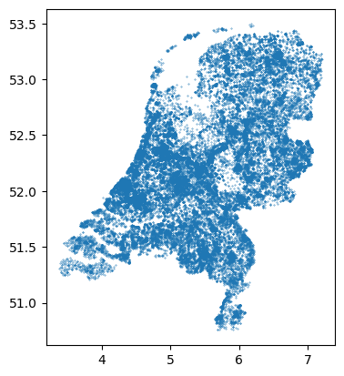
The points represents all the wells over the Netherlands. Since the wells are in the lat/lon coordinates. To make it comparable with fields, we need to first transfer the CRS to the “RD New” projection:
Now we would like to compare the wells with the cropped fields. We
can select the wells within the fields using the .clip
function:
OUTPUT
bro_id delivery_accountable_party quality_regime  ...
40744  GMW000000043703  27364178    IMBRO/A    ...
38728  GMW000000045818  27364178    IMBRO/A    ...
...                ...       ...        ...    ...
40174  GMW000000043963  27364178    IMBRO/A    ...
19445  GMW000000024992  50200097    IMBRO/A    ...
[79 rows x 40 columns]
After this selection, all the wells outside the fields are dropped. This takes a while to execute, because we are clipping a relatively large number of points with many polygons.
If we do not want a precise clipping, but rather have the points in the neighborhood of the fields, we will need to create another polygon, which is slightly bigger than the coverage of the field. To do this, we can increase the size of the field polygons, to make them overlap with each other, and then merge the overlapping polygons together.
We will first use the buffer function to increase field
size with a given distance. The unit of the
distance argument is the same as the CRS. Here we use a
50-meter buffer. Also notice that the .buffer function
produces a GeoSeries, so to keep the other columns, we
assign it to the GeoDataFrame as a geometry column.
PYTHON
buffer = fields.buffer(50)
fields_buffer = fields.copy()
fields_buffer['geometry'] = buffer
fields_buffer.plot()
To further simplify them, we can use the dissolve
function to dissolve the buffers into one:
All the fields will be dissolved into one multi-polygon, which can be
used to clip the wells.
In this way, we selected all wells within the 50m range of the
fields. It is also significantly faster than the previous
clip operation, since the number of polygons is much
smaller after dissolve.
Exercise: clip fields within 500m from the wells
This time, we will do a selection the other way around. Can you clip the field polygons (stored in fields_cropped.shp) with the 500m buffer of the wells (stored in brogmwvolledigeset.zip)? Please visualize the results.
Hint 1: The file
brogmwvolledigeset.zipis in CRS 4326. Don’t forget the CRS conversion.Hint 2:
brogmwvolledigeset.zipcontains all the wells in the Netherlands, which means it might be too big for the.buffer()function. To improve the performance, first crop it with the bounding box of the fields.
PYTHON
# Read in data
fields =  gpd.read_file("fields_cropped.shp")
wells = gpd.read_file("data/brogmwvolledigeset.zip")

# Crop points with bounding box
xmin, ymin, xmax, ymax = fields.total_bounds
wells = wells.to_crs(28992)
wells_cx = wells.cx[xmin-500:xmax+500, ymin-500:ymax+500]

# Create buffer
wells_cx_500mbuffer = wells_cx.copy()
wells_cx_500mbuffer['geometry'] = wells_cx.buffer(500)

# Clip
fields_clip_buffer = fields.clip(wells_cx_500mbuffer)
fields_clip_buffer.plot()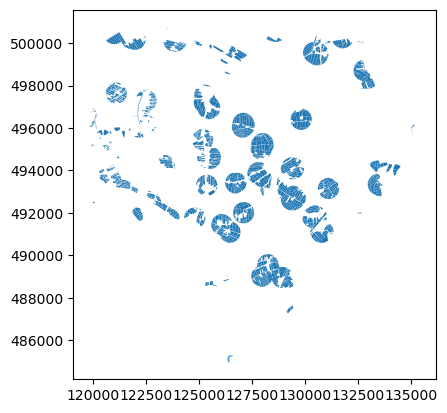
Spatially join the features
In the exercise, we clipped the fields polygons with the 500m buffers
of wells. The results from this clipping changed the shape of the
polygons. If we would like to keep the original shape of the fields, one
way is to use the sjoin function, which join two
GeoDataFrame’s on the basis of their spatial
relationship:
PYTHON
# Join fields and wells_cx_500mbuffer
fields_wells_buffer = fields.sjoin(wells_cx_500mbuffer)
print(fields_wells_buffer.shape)
OUTPUT
(11420, 46)This will result in a GeodataFrame of all possible
combinations of polygons and well buffers intersecting each other. Since
a polygon can fall into multiple buffers, there will be duplicated field
indexes in the results. To select the fields which intersects the well
buffers, we can first get the unique indexes, and use the
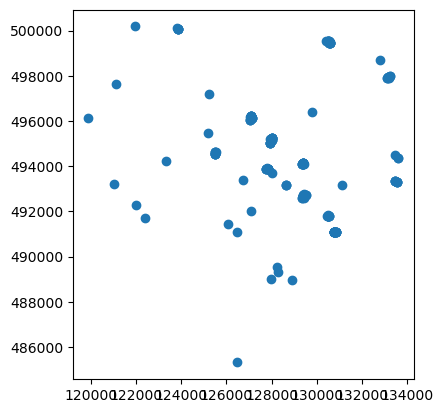
iloc indexer to select:
PYTHON
idx = fields_wells_buffer.index.unique()
fiedls_in_buffer = fields.iloc[idx]

fiedls_in_buffer.plot()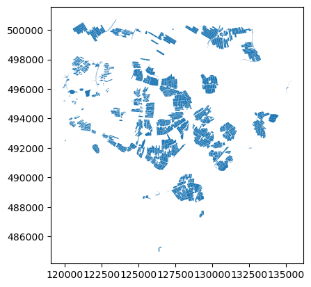
Modify the geometry of a GeoDataFrame
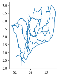
Exercise: Investigate the waterway lines
Now we will take a deeper look at the Dutch waterway lines:
waterways_nl. Let’s load the file
status_vaarweg.zip, and visualize it with the
plot() function. Can you tell what is wrong with this
vector file?
Axis ordering
According to the standards, the axis ordering for a CRS should follow the definition provided by the competent authority. For the commonly used EPSG:4326 geographic coordinate system, the EPSG defines the ordering as first latitude then longitude. However, in the GIS world, it is custom to work with coordinate tuples where the first component is aligned with the east/west direction and the second component is aligned with the north/south direction. Multiple software packages thus implement this convention also when dealing with EPSG:4326. As a result, one can encounter vector files that implement either convention - keep this in mind and always check your datasets!
Sometimes we need to modify the geometry of a
GeoDataFrame. For example, as we have seen in the previous
exercise Investigate the waterway lines, the latitude
and longitude are flipped in the vector data waterways_nl.
This error needs to be fixed before performing further analysis.
Let’s first take a look on what makes up the geometry
column of waterways_nl:
OUTPUT
0     LINESTRING (52.41810 4.84060, 52.42070 4.84090...
1     LINESTRING (52.11910 4.67450, 52.11930 4.67340...
2     LINESTRING (52.10090 4.25730, 52.10390 4.25530...
3     LINESTRING (53.47250 6.84550, 53.47740 6.83840...
4     LINESTRING (52.32270 5.14300, 52.32100 5.14640...
                            ...
86    LINESTRING (51.49270 5.39100, 51.48050 5.39160...
87    LINESTRING (52.15900 5.38510, 52.16010 5.38340...
88    LINESTRING (51.97340 4.12420, 51.97110 4.12220...
89    LINESTRING (52.11910 4.67450, 52.11850 4.67430...
90    LINESTRING (51.88940 4.61900, 51.89040 4.61350...
Name: geometry, Length: 91, dtype: geometry
Each row is a LINESTRING object. We can further zoom
into one of the rows, for example, the third row:
OUTPUT
LINESTRING (52.100900002 4.25730000099998, 52.1039 4.25529999999998, 52.111299999 4.24929999900002, 52.1274 4.23449999799999)
<class 'shapely.geometry.linestring.LineString'>
As we can see in the output, the LINESTRING object
contains a list of coordinates of the vertices. In our situation, we
would like to find a way to flip the x and y of every coordinates set. A
good way to look for the solution is to use the documentation
of the shapely package, since we are seeking to modify the
LINESTRING object. Here we are going to use the shapely.ops.transform
function, which applies a self-defined function to all coordinates of a
geometry.
PYTHON
import shapely

# Define a function flipping the x and y coordinate values
def flip(geometry):
    return shapely.ops.transform(lambda x, y: (y, x), geometry)

# Apply this function to all coordinates and all lines
geom_corrected = waterways_nl['geometry'].apply(flip)
Then we can update the geometry column with the
corrected geometry geom_corrected, and visualize it to
check:
PYTHON
# Update geometry
waterways_nl['geometry'] = geom_corrected

# Visualization
waterways_nl.plot()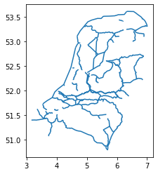
Now the waterways look good! We can save the vector data for later usage:
Key Points
- Load spatial objects into Python with
geopandas.read_file()function. - Spatial objects can be plotted directly with
GeoDataFrame’s.plot()method. - Crop spatial objects with
.cx[]indexer. - Convert CRS of spatial objects with
.to_crs(). - Select spatial features with
.clip(). - Create a buffer of spatial objects with
.buffer(). - Merge overlapping spatial objects with
.dissolve(). - Join spatial features spatially with
.sjoin().