Read and visualize raster data
Last updated on 2023-08-23 | Edit this page
Overview
Questions
- How is a raster represented by rioxarray?
- How do I read and plot raster data in Python?
- How can I handle missing data?
Objectives
- Describe the fundamental attributes of a raster dataset.
- Explore raster attributes and metadata using Python.
- Read rasters into Python using the
rioxarraypackage. - Visualize single/multi-band raster data.
Raster datasets have been introduced in Episode 1: Introduction to Raster Data. Here, we introduce the fundamental principles, packages and metadata/raster attributes for working with raster data in Python. We will also explore how Python handles missing and bad data values.
rioxarray
is the Python package we will use throughout this lesson to work with
raster data. It is based on the popular rasterio
package for working with rasters and xarray for
working with multi-dimensional arrays. rioxarray extends
xarray by providing top-level functions (e.g. the
open_rasterio function to open raster datasets) and by
adding a set of methods to the main objects of the xarray
package (the Dataset and the DataArray). These
additional methods are made available via the rio accessor
and become available from xarray objects after importing
rioxarray.
We will also use the pystac
package to load rasters from the search results we created in the
previous episode.
Introduce the Raster Data
We’ll continue from the results of the satellite image search that we
have carried out in an exercise from a
previous episode. We will load data starting from the
search.json file, using one scene from the search results
as an example to demonstrate data loading and visualization.
If you would like to work with the data for this lesson without
downloading data on-the-fly, you can download the raster data ahead of
time using this link. Save
the geospatial-python-raster-dataset.tar.gz file in your
current working directory, and extract the archive file by
double-clicking on it or by running the following command in your
terminal tar -zxvf geospatial-python-raster-dataset.tar.gz.
Use the file geospatial-python-raster-dataset/search.json
(instead of search.json) to get started with this
lesson.
This can be useful if you need to download the data ahead of time to work through the lesson offline, or if you want to work with the data in a different GIS.
Load a Raster and View Attributes
In the previous episode, we searched for Sentinel-2 images, and then
saved the search results to a file: search.json. This
contains the information on where and how to access the target images
from a remote repository. We can use the function
pystac.ItemCollection.from_file() to load the search
results as an Item list.
In the search results, we have 2 Item type objects,
corresponding to 4 Sentinel-2 scenes from March 26th and 28th in 2020.
We will focus on the first scene S2A_31UFU_20200328_0_L2A,
and load band nir09 (central wavelength 945 nm). We can
load this band using the function
rioxarray.open_rasterio(), via the Hypertext Reference
href (commonly referred to as a URL):
By calling the variable name in the jupyter notebook we can get a quick look at the shape and attributes of the data.
OUTPUT
<xarray.DataArray (band: 1, y: 1830, x: 1830)>
[3348900 values with dtype=uint16]
Coordinates:
  * band         (band) int64 1
  * x            (x) float64 6e+05 6.001e+05 6.002e+05 ... 7.097e+05 7.098e+05
  * y            (y) float64 5.9e+06 5.9e+06 5.9e+06 ... 5.79e+06 5.79e+06
    spatial_ref  int64 0
Attributes:
    _FillValue:    0.0
    scale_factor:  1.0
    add_offset:    0.0
The first call to rioxarray.open_rasterio() opens the
file from remote or local storage, and then returns a
xarray.DataArray object. The object is stored in a
variable, i.e. raster_ams_b9. Reading in the data with
xarray instead of rioxarray also returns a
xarray.DataArray, but the output will not contain the
geospatial metadata (such as projection information). You can use numpy
functions or built-in Python math operators on a
xarray.DataArray just like a numpy array. Calling the
variable name of the DataArray also prints out all of its
metadata information.
The output tells us that we are looking at an
xarray.DataArray, with 1 band,
1830 rows, and 1830 columns. We can also see
the number of pixel values in the DataArray, and the type
of those pixel values, which is unsigned integer (or
uint16). The DataArray also stores different
values for the coordinates of the DataArray. When using
rioxarray, the term coordinates refers to spatial
coordinates like x and y but also the
band coordinate. Each of these sequences of values has its
own data type, like float64 for the spatial coordinates and
int64 for the band coordinate.
This DataArray object also has a couple of attributes
that are accessed like .rio.crs, .rio.nodata,
and .rio.bounds(), which contain the metadata for the file
we opened. Note that many of the metadata are accessed as attributes
without (), but bounds() is a method (i.e. a
function in an object) and needs parentheses.
PYTHON
print(raster_ams_b9.rio.crs)
print(raster_ams_b9.rio.nodata)
print(raster_ams_b9.rio.bounds())
print(raster_ams_b9.rio.width)
print(raster_ams_b9.rio.height)
OUTPUT
EPSG:32631
0
(600000.0, 5790240.0, 709800.0, 5900040.0)
1830
1830
The Coordinate Reference System, or
raster_ams_b9.rio.crs, is reported as the string
EPSG:32631. The nodata value is encoded as 0
and the bounding box corners of our raster are represented by the output
of .bounds() as a tuple (like a list but you
can’t edit it). The height and width match what we saw when we printed
the DataArray, but by using .rio.width and
.rio.height we can access these values if we need them in
calculations.
We will be exploring this data throughout this episode. By the end of this episode, you will be able to understand and explain the metadata output.
Tip - Variable names
To improve code readability, file and object names should be used
that make it clear what is in the file. The data for this episode covers
Amsterdam, and is from Band 9, so we’ll use a naming convention of
raster_ams_b9.
Visualize a Raster
After viewing the attributes of our raster, we can examine the raw
values of the array with .values:
OUTPUT
array([[[    0,     0,     0, ...,  8888,  9075,  8139],
        [    0,     0,     0, ..., 10444, 10358,  8669],
        [    0,     0,     0, ..., 10346, 10659,  9168],
        ...,
        [    0,     0,     0, ...,  4295,  4289,  4320],
        [    0,     0,     0, ...,  4291,  4269,  4179],
        [    0,     0,     0, ...,  3944,  3503,  3862]]], dtype=uint16)
This can give us a quick view of the values of our array, but only at
the corners. Since our raster is loaded in python as a
DataArray type, we can plot this in one line similar to a
pandas DataFrame with DataArray.plot().
Nice plot! Notice that rioxarray helpfully allows us to
plot this raster with spatial coordinates on the x and y axis (this is
not the default in many cases with other functions or libraries).
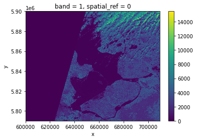
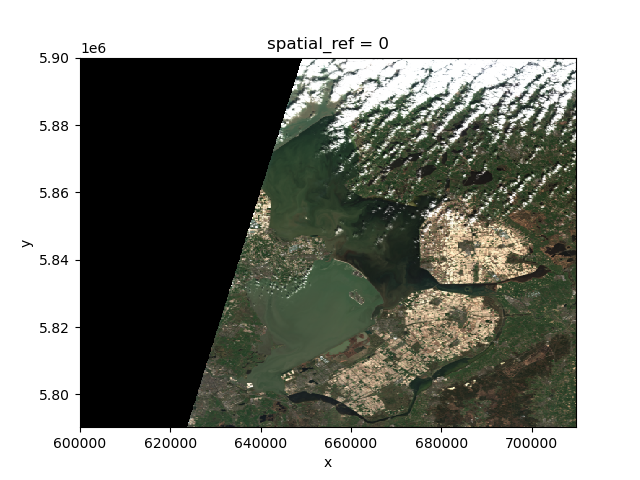
This plot shows the satellite measurement of the spectral band
nir09 for an area that covers part of the Netherlands.
According to the Sentinel-2
documentaion, this is a band with the central wavelength of 945nm,
which is sensitive to water vapor. It has a spatial resolution of 60m.
Note that the band=1 in the image title refers to the
ordering of all the bands in the DataArray, not the
Sentinel-2 band number 09 that we saw in the pystac search
results.
With a quick view of the image, we notice that half of the image is
blank, no data is captured. We also see that the cloudy pixels at the
top have high reflectance values, while the contrast of everything else
is quite low. This is expected because this band is sensitive to the
water vapor. However if one would like to have a better color contrast,
one can add the option robust=True, which displays values
between the 2nd and 98th percentile:
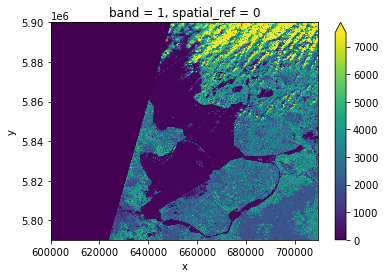
Now the color limit is set in a way fitting most of the values in the image. We have a better view of the ground pixels.
Tool Tip
The option robust=True always forces displaying values
between the 2nd and 98th percentile. Of course, this will not work for
every case. For a customized displaying range, you can also manually
specifying the keywords vmin and vmax. For
example ploting between 100 and 7000:
View Raster Coordinate Reference System (CRS) in Python
Another information that we’re interested in is the CRS, and it can
be accessed with .rio.crs. We introduced the concept of a
CRS in an earlier episode. Now we will see how
features of the CRS appear in our data file and what meanings they have.
We can view the CRS string associated with our DataArray’s
rio object using the crs attribute.
OUTPUT
EPSG:32631To print the EPSG code number as an int, we use the
.to_epsg() method:
OUTPUT
32631EPSG codes are great for succinctly representing a particular
coordinate reference system. But what if we want to see more details
about the CRS, like the units? For that, we can use pyproj,
a library for representing and working with coordinate reference
systems.
OUTPUT
<Derived Projected CRS: EPSG:32631>
Name: WGS 84 / UTM zone 31N
Axis Info [cartesian]:
- E[east]: Easting (metre)
- N[north]: Northing (metre)
Area of Use:
- name: Between 0°E and 6°E, northern hemisphere between equator and 84°N, onshore and offshore. Algeria. Andorra. Belgium. Benin. Burkina Faso. Denmark - North Sea. France. Germany - North Sea. Ghana. Luxembourg. Mali. Netherlands. Niger. Nigeria. Norway. Spain. Togo. United Kingdom (UK) - North Sea.
- bounds: (0.0, 0.0, 6.0, 84.0)
Coordinate Operation:
- name: UTM zone 31N
- method: Transverse Mercator
Datum: World Geodetic System 1984 ensemble
- Ellipsoid: WGS 84
- Prime Meridian: Greenwich
The CRS class from the pyproj library
allows us to create a CRS object with methods and
attributes for accessing specific information about a CRS, or the
detailed summary shown above.
A particularly useful attribute is area_of_use, which
shows the geographic bounds that the CRS is intended to be used.
OUTPUT
AreaOfUse(west=0.0, south=0.0, east=6.0, north=84.0, name='Between 0°E and 6°E, northern hemisphere between equator and 84°N, onshore and offshore. Algeria. Andorra. Belgium. Benin. Burkina Faso. Denmark - North Sea. France. Germany - North Sea. Ghana. Luxembourg. Mali. Netherlands. Niger. Nigeria. Norway. Spain. Togo. United Kingdom (UK) - North Sea.')Exercise: find the axes units of the CRS
What units are our data in? See if you can find a method to examine
this information using help(crs) or
dir(crs)
crs.axis_info tells us that the CRS for our raster has
two axis and both are in meters. We could also get this information from
the attribute raster_ams_b9.rio.crs.linear_units.
Understanding pyproj CRS Summary
Let’s break down the pieces of the pyproj CRS summary.
The string contains all of the individual CRS elements that Python or
another GIS might need, separated into distinct sections, and datum.
OUTPUT
<Derived Projected CRS: EPSG:32631>
Name: WGS 84 / UTM zone 31N
Axis Info [cartesian]:
- E[east]: Easting (metre)
- N[north]: Northing (metre)
Area of Use:
- name: Between 0°E and 6°E, northern hemisphere between equator and 84°N, onshore and offshore. Algeria. Andorra. Belgium. Benin. Burkina Faso. Denmark - North Sea. France. Germany - North Sea. Ghana. Luxembourg. Mali. Netherlands. Niger. Nigeria. Norway. Spain. Togo. United Kingdom (UK) - North Sea.
- bounds: (0.0, 0.0, 6.0, 84.0)
Coordinate Operation:
- name: UTM zone 31N
- method: Transverse Mercator
Datum: World Geodetic System 1984 ensemble
- Ellipsoid: WGS 84
- Prime Meridian: Greenwich- Name of the projection is UTM zone 31N (UTM has 60 zones, each 6-degrees of longitude in width). The underlying datum is WGS84.
- Axis Info: the CRS shows a Cartesian system with two axes, easting and northing, in meter units.
-
Area of Use: the projection is used for a
particular range of longitudes
0°E to 6°Ein the northern hemisphere (0.0°N to 84.0°N) - Coordinate Operation: the operation to project the coordinates (if it is projected) onto a cartesian (x, y) plane. Transverse Mercator is accurate for areas with longitudinal widths of a few degrees, hence the distinct UTM zones.
-
Datum: Details about the datum, or the reference
point for coordinates.
WGS 84andNAD 1983are common datums.NAD 1983is set to be replaced in 2022.
Note that the zone is unique to the UTM projection. Not all CRSs will have a zone. Below is a simplified view of US UTM zones.

Calculate Raster Statistics
It is useful to know the minimum or maximum values of a raster
dataset. We can compute these and other descriptive statistics with
min, max, mean, and
std.
PYTHON
print(raster_ams_b9.min())
print(raster_ams_b9.max())
print(raster_ams_b9.mean())
print(raster_ams_b9.std())
OUTPUT
<xarray.DataArray ()>
array(0, dtype=uint16)
Coordinates:
    spatial_ref  int64 0
<xarray.DataArray ()>
array(15497, dtype=uint16)
Coordinates:
    spatial_ref  int64 0
<xarray.DataArray ()>
array(1652.44009944)
Coordinates:
    spatial_ref  int64 0
<xarray.DataArray ()>
array(2049.16447495)
Coordinates:
    spatial_ref  int64 0
The information above includes a report of the min, max, mean, and
standard deviation values, along with the data type. If we want to see
specific quantiles, we can use xarray’s .quantile() method.
For example for the 25% and 75% quantiles:
OUTPUT
<xarray.DataArray (quantile: 2)>
array([   0., 2911.])
Coordinates:
  * quantile  (quantile) float64 0.25 0.75
Data Tip - NumPy methods
You could also get each of these values one by one using
numpy.
PYTHON
import numpy
print(numpy.percentile(raster_ams_b9, 25))
print(numpy.percentile(raster_ams_b9, 75))
OUTPUT
0.0
2911.0
You may notice that raster_ams_b9.quantile and
numpy.percentile didn’t require an argument specifying the
axis or dimension along which to compute the quantile. This is because
axis=None is the default for most numpy functions, and
therefore dim=None is the default for most xarray methods.
It’s always good to check out the docs on a function to see what the
default arguments are, particularly when working with multi-dimensional
image data. To do so, we can
usehelp(raster_ams_b9.quantile) or
?raster_ams_b9.percentile if you are using jupyter notebook
or jupyter lab.
Dealing with Missing Data
So far, we have visualized a band of a Sentinel-2 scene and
calculated its statistics. However, we need to take missing data into
account. Raster data often has a “no data value” associated with it and
for raster datasets read in by rioxarray. This value is
referred to as nodata. This is a value assigned to pixels
where data is missing or no data were collected. There can be different
cases that cause missing data, and it’s common for other values in a
raster to represent different cases. The most common example is missing
data at the edges of rasters.
By default the shape of a raster is always rectangular. So if we have a dataset that has a shape that isn’t rectangular, some pixels at the edge of the raster will have no data values. This often happens when the data were collected by a sensor which only flew over some part of a defined region.
As we have seen above, the nodata value of this dataset
(raster_ams_b9.rio.nodata) is 0. When we have plotted the
band data, or calculated statistics, the missing value was not
distinguished from other values. Missing data may cause some unexpected
results. For example, the 25th percentile we just calculated was 0,
probably reflecting the presence of a lot of missing data in the
raster.
To distinguish missing data from real data, one possible way is to
use nan to represent them. This can be done by specifying
masked=True when loading the raster:
One can also use the where function to select all the
pixels which are different from the nodata value of the
raster:
Either way will change the nodata value from 0 to
nan. Now if we compute the statistics again, the missing
data will not be considered:
print(raster_ams_b9.min())
print(raster_ams_b9.max())
print(raster_ams_b9.mean())
print(raster_ams_b9.std())
```python

```output
<xarray.DataArray ()>
array(8., dtype=float32)
Coordinates:
    spatial_ref  int64 0
<xarray.DataArray ()>
array(15497., dtype=float32)
Coordinates:
    spatial_ref  int64 0
<xarray.DataArray ()>
array(2477.405, dtype=float32)
Coordinates:
    spatial_ref  int64 0
<xarray.DataArray ()>
array(2061.9539, dtype=float32)
Coordinates:
    spatial_ref  int64 0
And if we plot the image, the nodata pixels are not
shown because they are not 0 anymore:
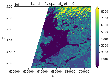
One should notice that there is a side effect of using
nan instead of 0 to represent the missing
data: the data type of the DataArray was changed from
integers to float. This need to be taken into consideration when the
data type matters in your application.
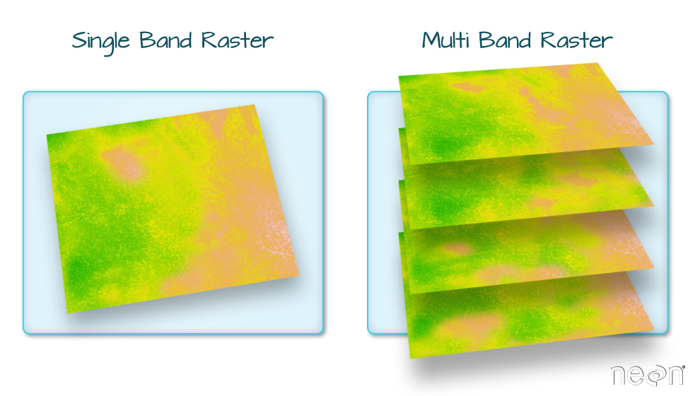
Raster Bands
So far we looked into a single band raster, i.e. the
nir09 band of a Sentinel-2 scene. However, to get a
smaller, non georeferenced version of the scene, one may also want to
visualize the true-color overview of the region. This is provided as a
multi-band raster – a raster dataset that contains more than one
band.
The overview asset in the Sentinel-2 scene is a
multiband asset. Similar to nir09, we can load it by:
PYTHON
raster_ams_overview = rioxarray.open_rasterio(items[0].assets['visual'].href, overview_level=3)
raster_ams_overview
OUTPUT
<xarray.DataArray (band: 3, y: 687, x: 687)>
[1415907 values with dtype=uint8]
Coordinates:
  * band         (band) int64 1 2 3
  * x            (x) float64 6.001e+05 6.002e+05 ... 7.096e+05 7.097e+05
  * y            (y) float64 5.9e+06 5.9e+06 5.9e+06 ... 5.79e+06 5.79e+06
    spatial_ref  int64 0
Attributes:
    AREA_OR_POINT:       Area
    OVR_RESAMPLING_ALG:  AVERAGE
    _FillValue:          0
    scale_factor:        1.0
    add_offset:          0.0
The band number comes first when GeoTiffs are read with the
.open_rasterio() function. As we can see in the
xarray.DataArray object, the shape is now
(band: 3, y: 687, x: 687), with three bands in the
band dimension. It’s always a good idea to examine the
shape of the raster array you are working with and make sure it’s what
you expect. Many functions, especially the ones that plot images, expect
a raster array to have a particular shape. One can also check the shape
using the .shape attribute:
OUTPUT
(3, 687, 687)One can visualize the multi-band data with the
DataArray.plot.imshow() function:
Note that the DataArray.plot.imshow() function makes
assumptions about the shape of the input DataArray, that since it has
three channels, the correct colormap for these channels is RGB. It does
not work directly on image arrays with more than 3 channels. One can
replace one of the RGB channels with another band, to make a false-color
image.
Exercise: set the plotting aspect ratio
As seen in the figure above, the true-color image is stretched. Let’s
visualize it with the right aspect ratio. You can use the documentation
of DataArray.plot.imshow().
Since we know the height/width ratio is 1:1 (check the
rio.height and rio.width attributes), we can
set the aspect ratio to be 1. For example, we can choose the size to be
5 inches, and set aspect=1. Note that according to the documentation
of DataArray.plot.imshow(), when specifying the
aspect argument, size also needs to be
provided.

Key Points
-
rioxarrayandxarrayare for working with multidimensional arrays like pandas is for working with tabular data. -
rioxarraystores CRS information as a CRS object that can be converted to an EPSG code or PROJ4 string. - Missing raster data are filled with nodata values, which should be handled with care for statistics and visualization.