Access satellite imagery using Python
Last updated on 2026-01-13 | Edit this page
Overview
Questions
- Where can I find open-access satellite data?
- How do I search for satellite imagery with the STAC API?
- How do I fetch remote raster datasets using Python?
Objectives
- Search public STAC repositories of satellite imagery using Python.
- Inspect search result’s metadata.
- Download (a subset of) the assets available for a satellite scene.
- Open satellite imagery as raster data and save it to disk.
Considerations for the position of this episode in the workshop
When this workshop is taught to learners with limited prior knowledge of Python, it might be better to place this episode after episode 11 and before episode 12. This episode contains an introduction to working with APIs and dictionaries, which can be perceived as challenging by some learners. Another consideration for placing this episode later in the workshop is when it is taught to learners with prior GIS knowledge who want to perform GIS-like operations with data they have already collected or for learners interested in working with raster data but less interested in satellite images.
Introduction
A number of satellites take snapshots of the Earth’s surface from space. The images recorded by these remote sensors represent a very precious data source for any activity that involves monitoring changes on Earth. Satellite imagery is typically provided in the form of geospatial raster data, with the measurements in each grid cell (“pixel”) being associated to accurate geographic coordinate information.
In this episode we will explore how to access open satellite data using Python. In particular, we will consider the Sentinel-2 data collection that is hosted on Amazon Web Services (AWS). This dataset consists of multi-band optical images acquired by the constellation of two satellites from the Sentinel-2 mission and it is continuously updated with new images.
Search for satellite imagery
The SpatioTemporal Asset Catalog (STAC) specification
Current sensor resolutions and satellite revisit periods are such that terabytes of data products are added daily to the corresponding collections. Such datasets cannot be made accessible to users via full-catalog download. Therefore, space agencies and other data providers often offer access to their data catalogs through interactive Graphical User Interfaces (GUIs), see for instance the Copernicus Browser for the Sentinel missions. Accessing data via a GUI is a nice way to explore a catalog and get familiar with its content, but it represents a heavy and error-prone task that should be avoided if carried out systematically to retrieve data.
A service that offers programmatic access to the data enables users to reach the desired data in a more reliable, scalable and reproducible manner. An important element in the software interface exposed to the users, which is generally called the Application Programming Interface (API), is the use of standards. Standards, in fact, can significantly facilitate the reusability of tools and scripts across datasets and applications.
The SpatioTemporal Asset Catalog (STAC) specification is an emerging standard for describing geospatial data. By organizing metadata in a form that adheres to the STAC specifications, data providers make it possible for users to access data from different missions, instruments and collections using the same set of tools.
Search a STAC catalog
The STAC browser is a good starting point to discover available datasets, as it provides an up-to-date list of existing STAC catalogs. From the list, let’s click on the “Earth Search” catalog, i.e. the access point to search the archive of Sentinel-2 images hosted on AWS.
Exercise: Discover a STAC catalog
Let’s take a moment to explore the Earth Search STAC catalog, which is the catalog indexing the Sentinel-2 collection that is hosted on AWS. We can interactively browse this catalog using the STAC browser at this link.
- Open the link in your web browser. Which (sub-)catalogs are available?
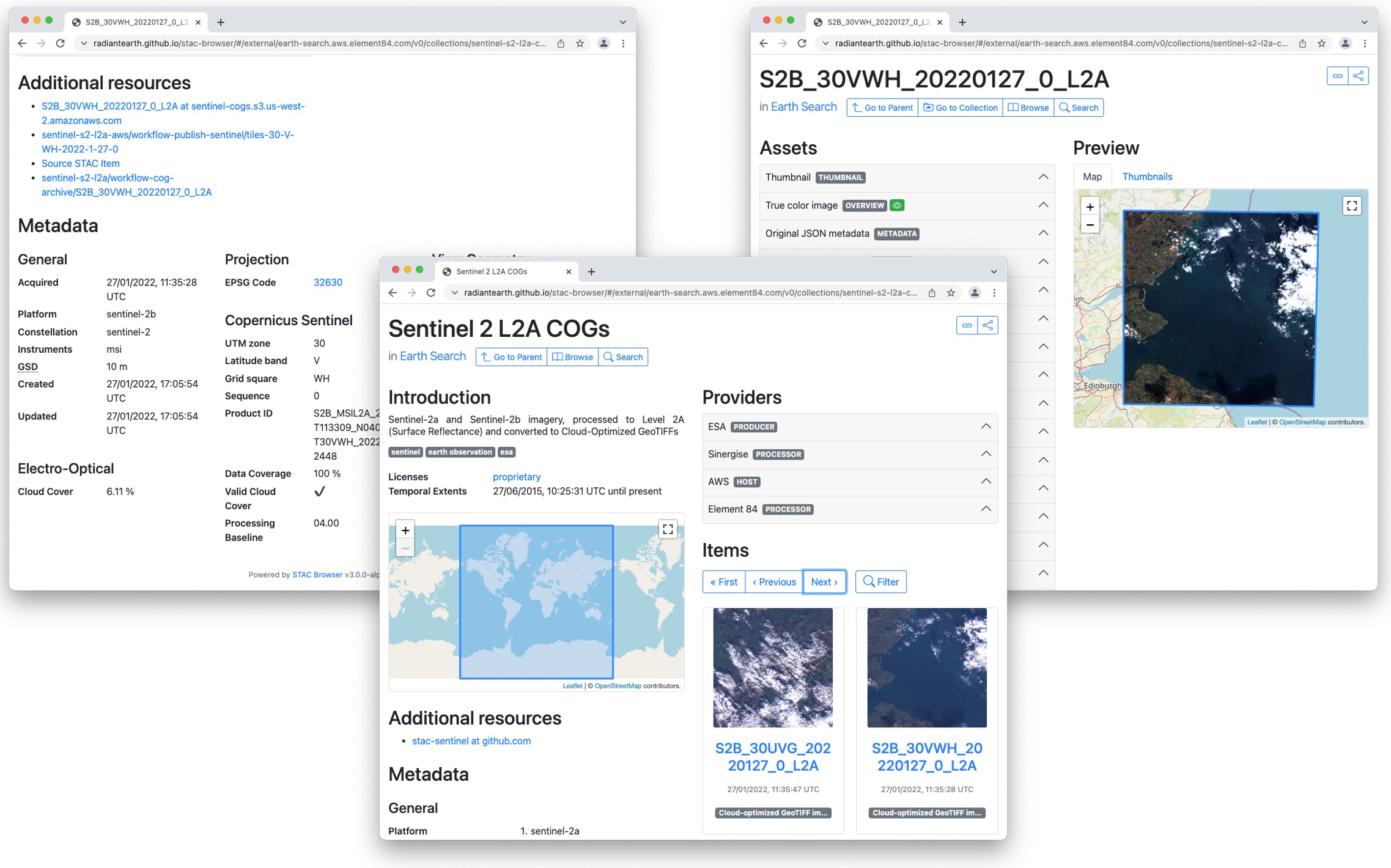
- Open the Sentinel-2 Level 2A collection, and select one item from the list. Each item corresponds to a satellite “scene”, i.e. a portion of the footage recorded by the satellite at a given time. Have a look at the metadata fields and the list of assets. What kind of data do the assets represent?
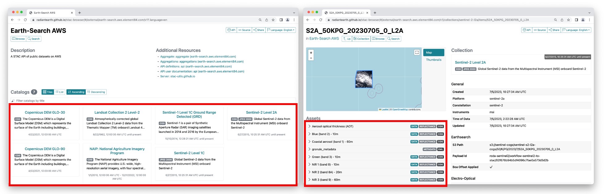
- 8 sub-catalogs are available. In the STAC nomenclature, these are actually “collections”, i.e. catalogs with additional information about the elements they list: spatial and temporal extents, license, providers, etc. Among the available collections, we have Landsat Collection 2, Level-2 and Sentinel-2 Level 2A (see left screenshot in the figure above).
- When you select the Sentinel-2 Level 2A collection, and randomly choose one of the items from the list, you should find yourself on a page similar to the right screenshot in the figure above. On the left side you will find a list of the available assets: overview images (thumbnail and true color images), metadata files and the “real” satellite images, one for each band captured by the Multispectral Instrument on board Sentinel-2.
When opening a catalog with the STAC browser, you can access the API URL by clicking on the “Source” button on the top right of the page. By using this URL, you have access to the catalog content and, if supported by the catalog, to the functionality of searching its items. For the Earth Search STAC catalog the API URL is:
You can query a STAC API endpoint from Python using the pystac_client
library. To do so we will first import Client from
pystac_client and use the method
open from the Client object:
For this episode we will focus at scenes belonging to the
sentinel-2-l2a collection. This dataset is useful for our
case and includes Sentinel-2 data products pre-processed at level 2A
(bottom-of-atmosphere reflectance).
In order to see which collections are available in the provided
api_url the get_collections
method can be used on the Client object.
To print the collections we can make a for loop doing:
OUTPUT
<CollectionClient id=cop-dem-glo-30>
<CollectionClient id=naip>
<CollectionClient id=sentinel-2-l2a>
<CollectionClient id=sentinel-2-l1c>
<CollectionClient id=cop-dem-glo-90>
<CollectionClient id=landsat-c2-l2>
<CollectionClient id=sentinel-1-grd>
<CollectionClient id=sentinel-2-c1-l2a>
As said, we want to focus to the sentinel-2-l2a
collection. To do so, we set this collection into a variable:
The data in this collection is stored in the Cloud Optimized GeoTIFF (COG) format and as JPEG2000 images. In this episode we will focus at COGs, as these offer useful functionalities for our purpose.
Cloud Optimized GeoTIFFs
Cloud Optimized GeoTIFFs (COGs) are regular GeoTIFF files with some additional features that make them ideal to be employed in the context of cloud computing and other web-based services. This format builds on the widely-employed GeoTIFF format, already introduced in Episode 1: Introduction to Raster Data. In essence, COGs are regular GeoTIFF files with a special internal structure. One of the features of COGs is that data is organized in “blocks” that can be accessed remotely via independent HTTP requests. Data users can thus access the only blocks of a GeoTIFF that are relevant for their analysis, without having to download the full file. In addition, COGs typically include multiple lower-resolution versions of the original image, called “overviews”, which can also be accessed independently. By providing this “pyramidal” structure, users that are not interested in the details provided by a high-resolution raster can directly access the lower-resolution versions of the same image, significantly saving on the downloading time. More information on the COG format can be found here.
In order to get data for a specific location you can add longitude
latitude coordinates (World Geodetic System 1984 EPSG:4326) in your
request. In order to do so we are using the shapely library
to define a geometrical point. Below we have included a point on the
island of Rhodes, which is the location of interest for our case study
(i.e. Longitude: 27.95 | Latitude 36.20).
PYTHON
from shapely.geometry import Point
point = Point(27.95, 36.20)  # Coordinates of a point on Rhodes
Note: at this stage, we are only dealing with metadata, so no image
is going to be downloaded yet. But even metadata can be quite bulky if a
large number of scenes match our search! For this reason, we limit the
search by the intersection of the point (by setting the parameter
intersects) and assign the collection (by setting the
parameter collections). More information about the possible
parameters to be set can be found in the pystac_client
documentation for the Client’s
search method.
We now set up our search of satellite images in the following way:
Now we submit the query in order to find out how many scenes match our search criteria with the parameters assigned above (please note that this output can be different as more data is added to the catalog to when this episode was created):
OUTPUT
611You will notice that more than 500 scenes match our search criteria. We are however interested in the period right before and after the wildfire of Rhodes. In the following exercise you will therefore have to add a time filter to our search criteria to narrow down our search for images of that period.
Exercise: Search satellite scenes with a time filter
Search for all the available Sentinel-2 scenes in the
sentinel-2-c1-l2a collection that have been recorded
between 1st of July 2023 and 31st of August 2023 (few weeks before and
after the time in which the wildfire took place).
Hint: You can find the input argument and the required syntax in the
documentation of client.search (which you can access from
Python or online)
How many scenes are available?
Now that we have added a time filter, we retrieve the metadata of the
search results by calling the method item_collection:
The variable items is an ItemCollection
object. More information can be found at the pystac
documentation
Now let us check the size using len:
OUTPUT
12which is consistent with the number of scenes matching our search
results as found with search.matched(). We can iterate over
the returned items and print these to show their IDs:
OUTPUT
<Item id=S2A_35SNA_20230827_0_L2A>
<Item id=S2B_35SNA_20230822_0_L2A>
<Item id=S2A_35SNA_20230817_0_L2A>
<Item id=S2B_35SNA_20230812_0_L2A>
<Item id=S2A_35SNA_20230807_0_L2A>
<Item id=S2B_35SNA_20230802_0_L2A>
<Item id=S2A_35SNA_20230728_0_L2A>
<Item id=S2B_35SNA_20230723_0_L2A>
<Item id=S2A_35SNA_20230718_0_L2A>
<Item id=S2B_35SNA_20230713_0_L2A>
<Item id=S2A_35SNA_20230708_0_L2A>
<Item id=S2B_35SNA_20230703_0_L2A>
Each of the items contains information about the scene geometry, its
acquisition time, and other metadata that can be accessed as a
dictionary from the properties attribute. To see which
information Item objects can contain you can have a look at the pystac
documentation.
Let us inspect the metadata associated with the first item of the search results. Let us first look at the collection date of the first item::
OUTPUT
2023-08-27 09:00:21.327000+00:00Let us now look at the geometry and other properties as well.
OUTPUT
{'type': 'Polygon', 'coordinates': [[[27.290401625602243, 37.04621863329741], [27.23303872472207, 36.83882218126937], [27.011145718480538, 36.05673246264742], [28.21878905911668, 36.05053734221328], [28.234426643135546, 37.04015200857309], [27.290401625602243, 37.04621863329741]]]}
{'created': '2023-08-27T18:15:43.106Z', 'platform': 'sentinel-2a', 'constellation': 'sentinel-2', 'instruments': ['msi'], 'eo:cloud_cover': 0.955362, 'proj:epsg': 32635, 'mgrs:utm_zone': 35, 'mgrs:latitude_band': 'S', 'mgrs:grid_square': 'NA', 'grid:code': 'MGRS-35SNA', 'view:sun_azimuth': 144.36354987218, 'view:sun_elevation': 59.06665363921, 's2:degraded_msi_data_percentage': 0.0126, 's2:nodata_pixel_percentage': 12.146327, 's2:saturated_defective_pixel_percentage': 0, 's2:dark_features_percentage': 0.249403, 's2:cloud_shadow_percentage': 0.237454, 's2:vegetation_percentage': 6.073786, 's2:not_vegetated_percentage': 18.026696, 's2:water_percentage': 74.259061, 's2:unclassified_percentage': 0.198216, 's2:medium_proba_clouds_percentage': 0.613614, 's2:high_proba_clouds_percentage': 0.341423, 's2:thin_cirrus_percentage': 0.000325, 's2:snow_ice_percentage': 2.3e-05, 's2:product_type': 'S2MSI2A', 's2:processing_baseline': '05.09', 's2:product_uri': 'S2A_MSIL2A_20230827T084601_N0509_R107_T35SNA_20230827T115803.SAFE', 's2:generation_time': '2023-08-27T11:58:03.000000Z', 's2:datatake_id': 'GS2A_20230827T084601_042718_N05.09', 's2:datatake_type': 'INS-NOBS', 's2:datastrip_id': 'S2A_OPER_MSI_L2A_DS_2APS_20230827T115803_S20230827T085947_N05.09', 's2:granule_id': 'S2A_OPER_MSI_L2A_TL_2APS_20230827T115803_A042718_T35SNA_N05.09', 's2:reflectance_conversion_factor': 0.978189079756816, 'datetime': '2023-08-27T09:00:21.327000Z', 's2:sequence': '0', 'earthsearch:s3_path': 's3://sentinel-cogs/sentinel-s2-l2a-cogs/35/S/NA/2023/8/S2A_35SNA_20230827_0_L2A', 'earthsearch:payload_id': 'roda-sentinel2/workflow-sentinel2-to-stac/af0287974aaa3fbb037c6a7632f72742', 'earthsearch:boa_offset_applied': True, 'processing:software': {'sentinel2-to-stac': '0.1.1'}, 'updated': '2023-08-27T18:15:43.106Z'}
You can access items from the properties dictionary as
usual in Python. For instance, for the EPSG code of the projected
coordinate system:
Exercise: Search satellite scenes using metadata filters
Let’s add a filter on the cloud cover to select the only scenes with less than 1% cloud coverage. How many scenes do now match our search?
Hint: generic metadata filters can be implemented via the
query input argument of client.search, which
requires the following syntax (see docs):
query=['<property><operator><value>'].
Once we are happy with our search, we save the search results in a file:
This creates a file in GeoJSON format, which we can reuse here and in the next episodes. Note that this file contains the metadata of the files that meet out criteria. It does not include the data itself, only their metadata.
To load the saved search results as a ItemCollection we
can use pystac.ItemCollection.from_file().
Through this, we are instructing Python to use the
from_file method of the ItemCollection class
from the pystac library to load data from the specified
GeoJSON file:
The loaded item collection (items_loaded) is equivalent
to the one returned earlier by search.item_collection()
(items). You can thus perform the same actions on it: you
can check the number of items (len(items_loaded)), you can
loop over items (for item in items_loaded: ...), and you
can access individual elements using their index
(items_loaded[0]).
Access the assets
So far we have only discussed metadata - but how can one get to the
actual images of a satellite scene (the “assets” in the STAC
nomenclature)? These can be reached via links that are made available
through the item’s attribute assets. Let’s focus on the
last item in the collection: this is the oldest in time, and it thus
corresponds to an image taken before the wildfires.
OUTPUT
dict_keys(['aot', 'blue', 'coastal', 'granule_metadata', 'green', 'nir', 'nir08', 'nir09', 'red', 'rededge1', 'rededge2', 'rededge3', 'scl', 'swir16', 'swir22', 'thumbnail', 'tileinfo_metadata', 'visual', 'wvp', 'aot-jp2', 'blue-jp2', 'coastal-jp2', 'green-jp2', 'nir-jp2', 'nir08-jp2', 'nir09-jp2', 'red-jp2', 'rededge1-jp2', 'rededge2-jp2', 'rededge3-jp2', 'scl-jp2', 'swir16-jp2', 'swir22-jp2', 'visual-jp2', 'wvp-jp2'])We can print a minimal description of the available assets:
OUTPUT
aot: Aerosol optical thickness (AOT)
blue: Blue (band 2) - 10m
coastal: Coastal aerosol (band 1) - 60m
granule_metadata: None
green: Green (band 3) - 10m
nir: NIR 1 (band 8) - 10m
nir08: NIR 2 (band 8A) - 20m
nir09: NIR 3 (band 9) - 60m
red: Red (band 4) - 10m
rededge1: Red edge 1 (band 5) - 20m
rededge2: Red edge 2 (band 6) - 20m
rededge3: Red edge 3 (band 7) - 20m
scl: Scene classification map (SCL)
swir16: SWIR 1 (band 11) - 20m
swir22: SWIR 2 (band 12) - 20m
thumbnail: Thumbnail image
tileinfo_metadata: None
visual: True color image
wvp: Water vapour (WVP)
aot-jp2: Aerosol optical thickness (AOT)
blue-jp2: Blue (band 2) - 10m
coastal-jp2: Coastal aerosol (band 1) - 60m
green-jp2: Green (band 3) - 10m
nir-jp2: NIR 1 (band 8) - 10m
nir08-jp2: NIR 2 (band 8A) - 20m
nir09-jp2: NIR 3 (band 9) - 60m
red-jp2: Red (band 4) - 10m
rededge1-jp2: Red edge 1 (band 5) - 20m
rededge2-jp2: Red edge 2 (band 6) - 20m
rededge3-jp2: Red edge 3 (band 7) - 20m
scl-jp2: Scene classification map (SCL)
swir16-jp2: SWIR 1 (band 11) - 20m
swir22-jp2: SWIR 2 (band 12) - 20m
visual-jp2: True color image
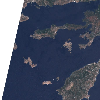
wvp-jp2: Water vapour (WVP)Among the other data files, assets include multiple raster data files (one per optical band, as acquired by the multi-spectral instrument), a thumbnail, a true-color image (“visual”), instrument metadata and scene-classification information (“SCL”). Let’s get the URL link to the thumbnail, which gives us a glimpse of the Sentinel-2 scene:
OUTPUT
https://sentinel-cogs.s3.us-west-2.amazonaws.com/sentinel-s2-l2a-cogs/35/S/NA/2023/7/S2A_35SNA_20230708_0_L2A/thumbnail.jpgThis can be used to download the corresponding file:
For comparison, we can check out the thumbnail of the most recent scene of the sequence considered (i.e. the first item in the item collection), which has been taken after the wildfires:
OUTPUT
https://sentinel-cogs.s3.us-west-2.amazonaws.com/sentinel-s2-l2a-cogs/35/S/NA/2023/8/S2A_35SNA_20230827_0_L2A/thumbnail.jpg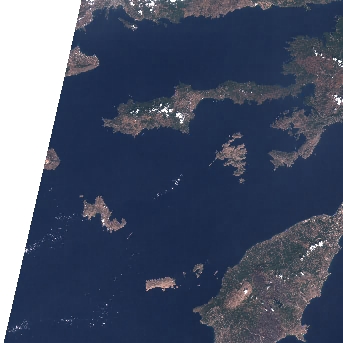
From the thumbnails alone we can already observe some dark spots on the island of Rhodes at the bottom right of the image!
In order to open the high-resolution satellite images and investigate
the scenes in more detail, we will be using the rioxarray
library. Note that this library can both work with local and remote
raster data. At this moment, we will only quickly look at the
functionality of this library. We will learn more about it in the next
episode.
Now let us focus on the red band by accessing the item
red from the assets dictionary and get the Hypertext
Reference (also known as URL) attribute using .href after
the item selection.
For now we are using rioxarray to open the raster file.
PYTHON
import rioxarray
red_href = assets["red"].href
red = rioxarray.open_rasterio(red_href)
print(red)
OUTPUT
<xarray.DataArray (band: 1, y: 10980, x: 10980)> Size: 241MB
[120560400 values with dtype=uint16]
Coordinates:
  * band         (band) int32 4B 1
  * x            (x) float64 88kB 5e+05 5e+05 5e+05 ... 6.098e+05 6.098e+05
  * y            (y) float64 88kB 4.1e+06 4.1e+06 4.1e+06 ... 3.99e+06 3.99e+06
    spatial_ref  int32 4B 0
Attributes:
    AREA_OR_POINT:       Area
    OVR_RESAMPLING_ALG:  AVERAGE
    _FillValue:          0
    scale_factor:        1.0
    add_offset:          0.0
Now we want to save the data to our local machine using the to_raster method:
That might take a while, given there are over 10000 x 10000 = a hundred million pixels in the 10-meter NIR band. But we can take a smaller subset before downloading it. Because the raster is a COG, we can download just what we need!
In order to do that, we are using rioxarray´s clip_box
with which you can set a bounding box defining the area you want.
Next, we save the subset using to_raster again.
The difference is 241 Megabytes for the full image vs less than 10 Megabytes for the subset.
Exercise: Downloading Landsat 8 Assets
In this exercise we put in practice all the skills we have learned in
this episode to retrieve images from a different mission: Landsat 8. In
particular, we browse images from the Harmonized Landsat
Sentinel-2 (HLS) project, which provides images from NASA’s Landsat
8 and ESA’s Sentinel-2 that have been made consistent with each other.
The HLS catalog is indexed in the NASA Common Metadata Repository (CMR)
and it can be accessed from the STAC API endpoint at the following URL:
https://cmr.earthdata.nasa.gov/stac/LPCLOUD.
- Using
pystac_client, search for all assets of the Landsat 8 collection (HLSL30.v2.0) from February to March 2021, intersecting the point with longitude/latitute coordinates (-73.97, 40.78) deg. - Visualize an item’s thumbnail (asset key
browse).
PYTHON
# connect to the STAC endpoint
cmr_api_url = "https://cmr.earthdata.nasa.gov/stac/LPCLOUD"
client = Client.open(cmr_api_url)

# setup search
search = client.search(
    collections=["HLSL30.v2.0"],
    intersects=Point(-73.97, 40.78),
    datetime="2021-02-01/2021-03-30",
) # nasa cmr cloud cover filtering is currently broken: https://github.com/nasa/cmr-stac/issues/239

# retrieve search results
items = search.item_collection()
print(len(items))
OUTPUT
5PYTHON
items_sorted = sorted(items, key=lambda x: x.properties["eo:cloud_cover"]) # sorting and then selecting by cloud cover
item = items_sorted[0]
print(item)
OUTPUT
<Item id=HLS.L30.T18TWL.2021039T153324.v2.0>OUTPUT
'https://data.lpdaac.earthdatacloud.nasa.gov/lp-prod-public/HLSL30.020/HLS.L30.T18TWL.2021039T153324.v2.0/HLS.L30.T18TWL.039T153324.v2.0.jpg'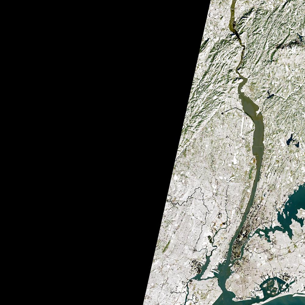
Public catalogs, protected data
Publicly accessible catalogs and STAC endpoints do not necessarily imply publicly accessible data. Data providers, in fact, may limit data access to specific infrastructures and/or require authentication. For instance, the NASA CMR STAC endpoint considered in the last exercise offers publicly accessible metadata for the HLS collection, but most of the linked assets are available only for registered users (the thumbnail is publicly accessible).
The authentication procedure for dataset with restricted access might differ depending on the data provider. For the NASA CMR, follow these steps in order to access data using Python:
- Create a NASA Earthdata login account here;
- Set up a netrc file with your credentials, e.g. by using this script;
- Define the following environment variables:
- Accessing satellite images via the providers’ API enables a more reliable and scalable data retrieval.
- STAC catalogs can be browsed and searched using the same tools and scripts.
-
rioxarrayallows you to open and download remote raster files.