All Images
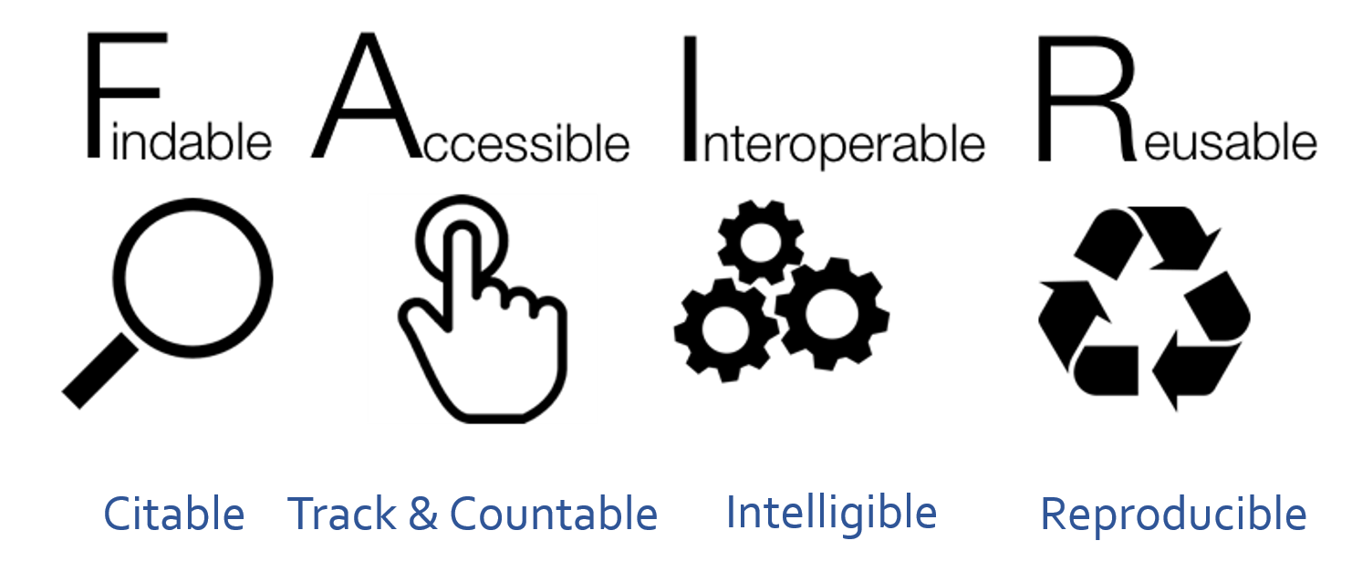
Introduction to Open Science and FAIR principles
Figure 1
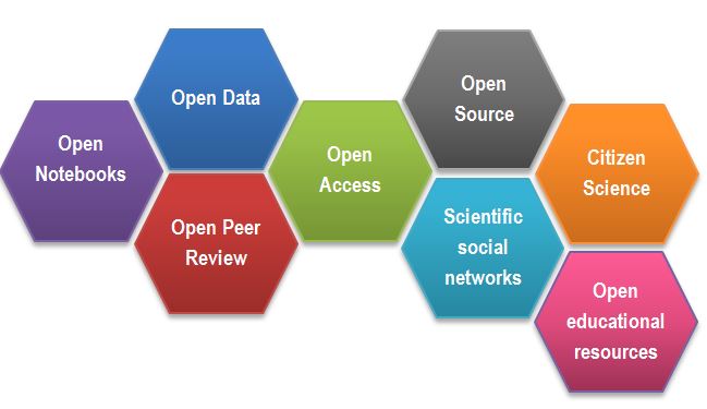
Figure 2
Figure 3
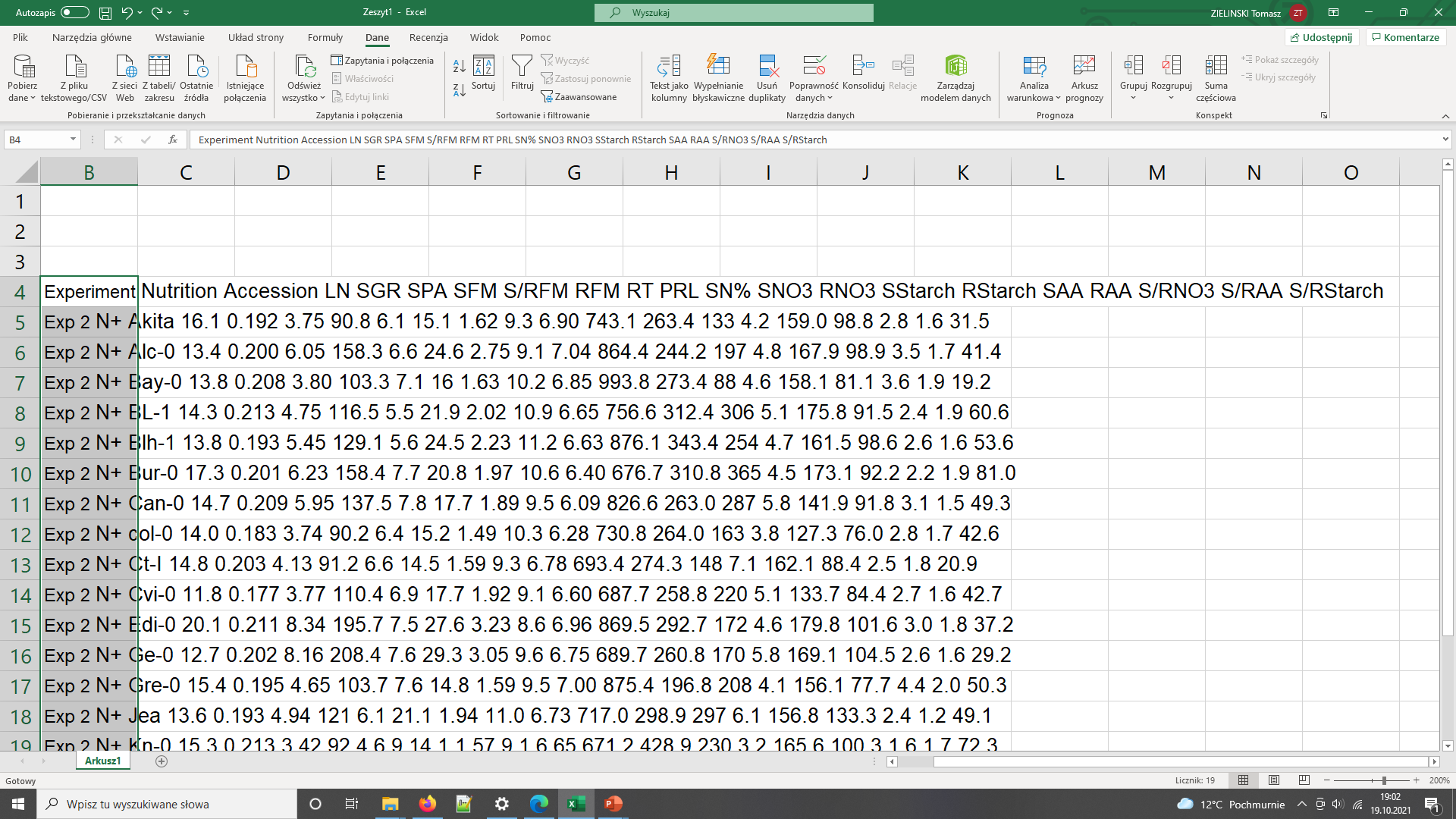
Data needs parsing after coping to Excel
The same data copied to Excel with polish locale has been converted to dates
Figure 4
 After SangyaPundir
Introduction to metadata
Figure 1
 Figure credits: María Eugenia Goya
Figure 2
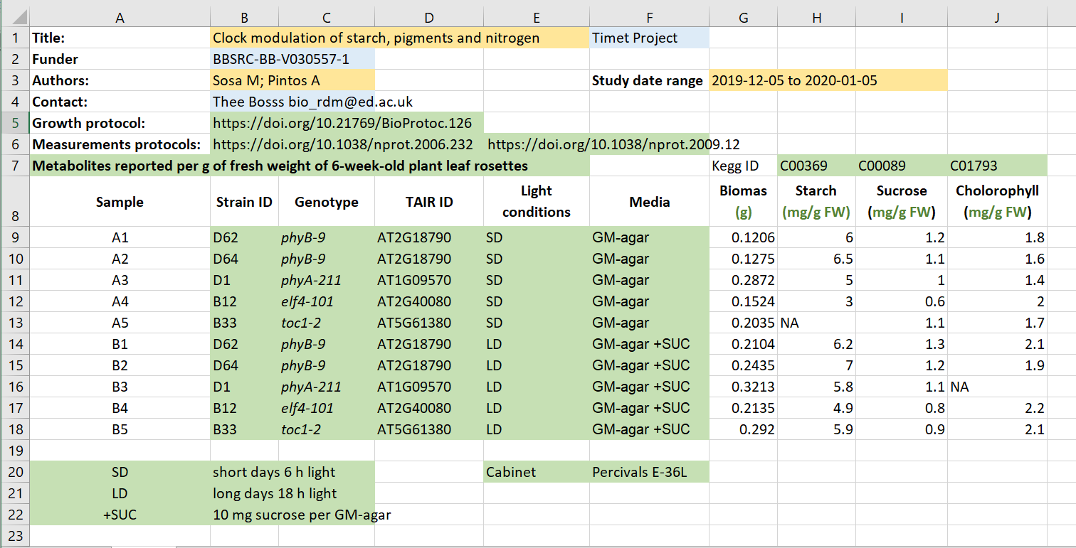
Figure credits: Tomasz Zielinski and Andrés Romanowski
Figure 3
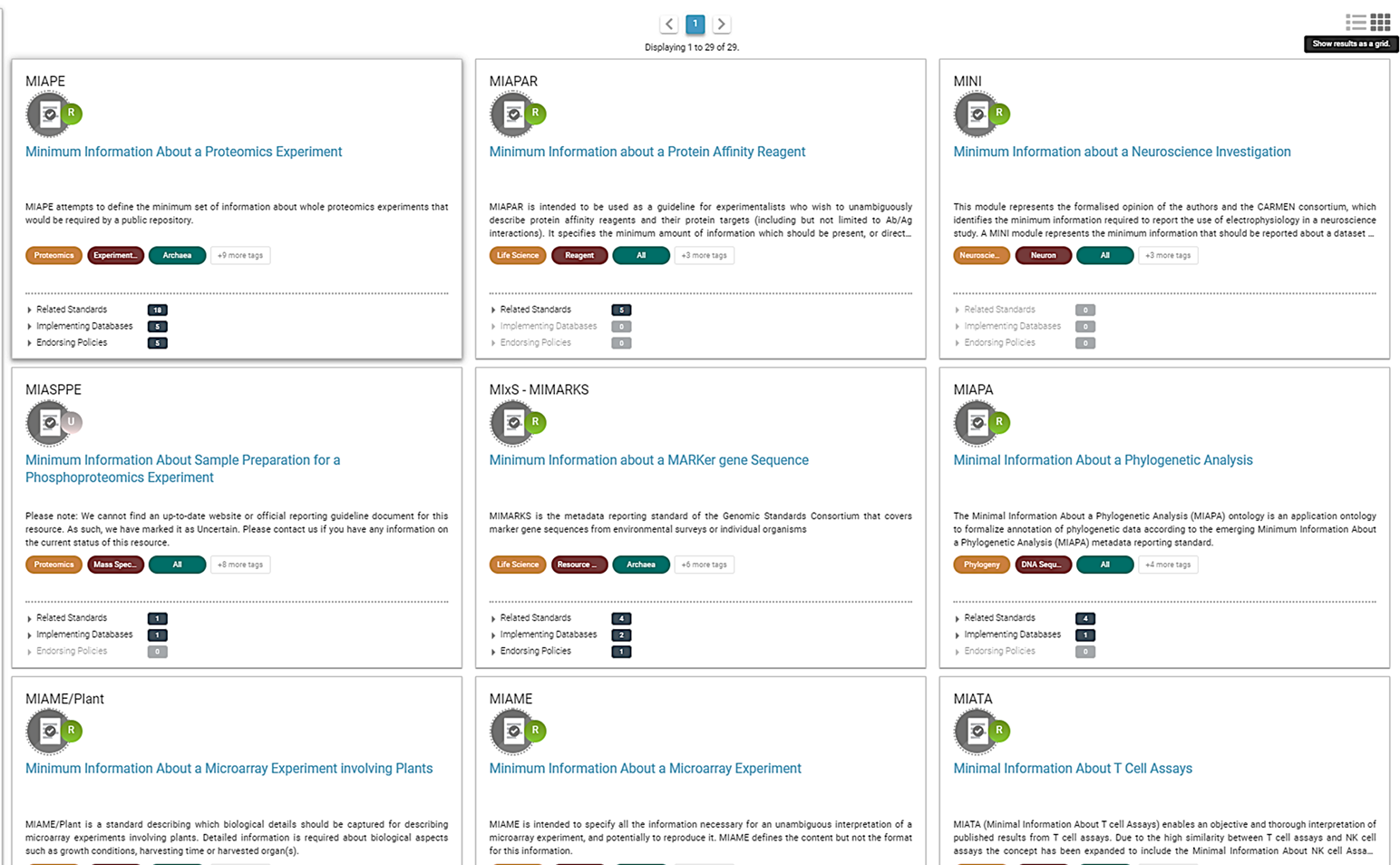
Figure. Some of the MIBBI minimum information standards from
fairsharing.org
Tidy (meta)data tables
Figure 1
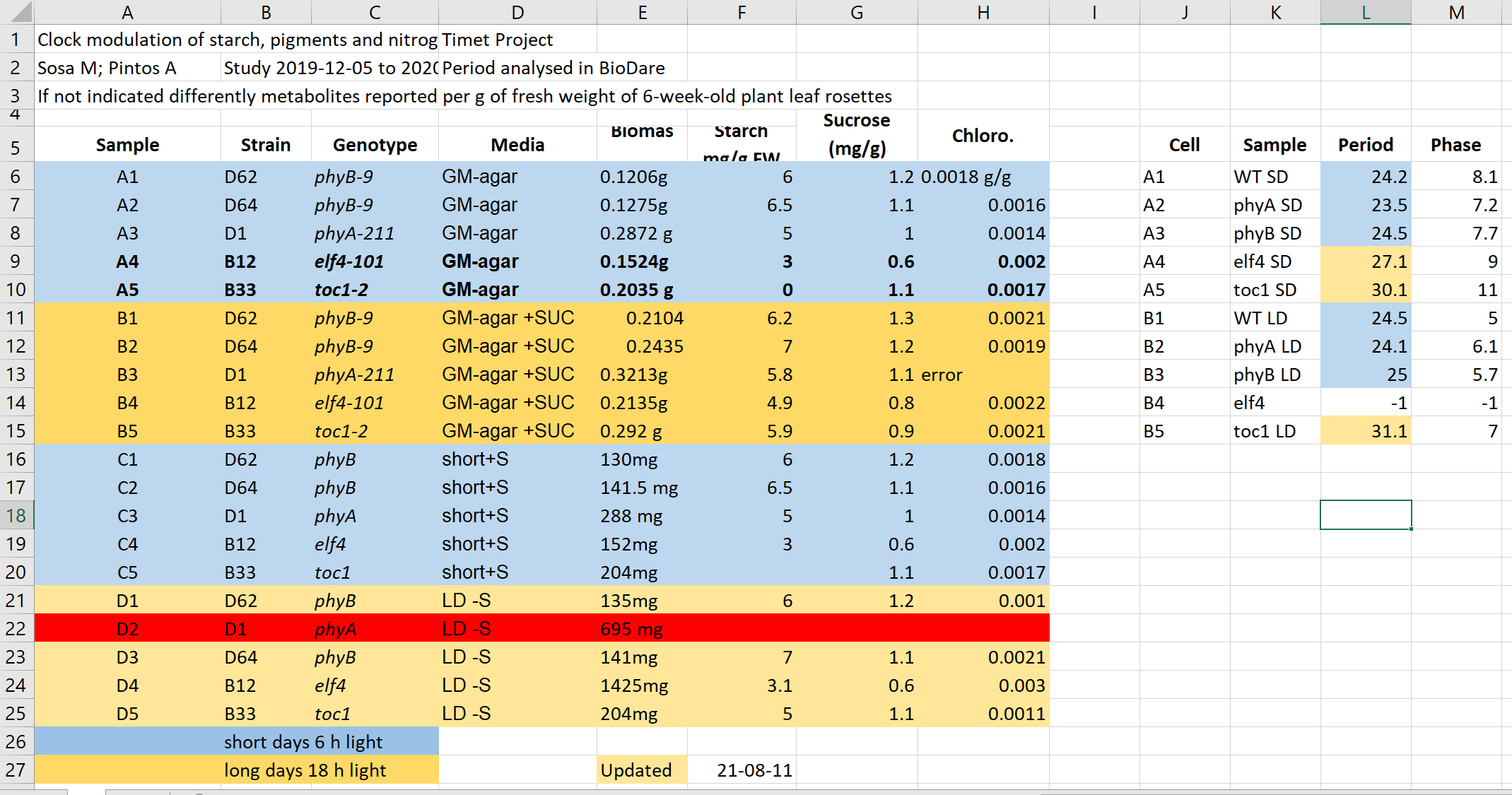
Figure 2
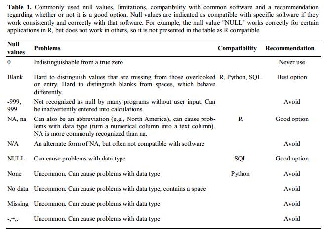
Figure 3
Working with files
Figure 1
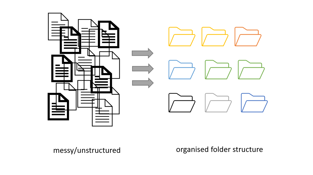 Figure credits: Andrés
Romanowski
Figure credits: Andrés
Romanowski
Figure 2
Have a look at the four different folder structures.
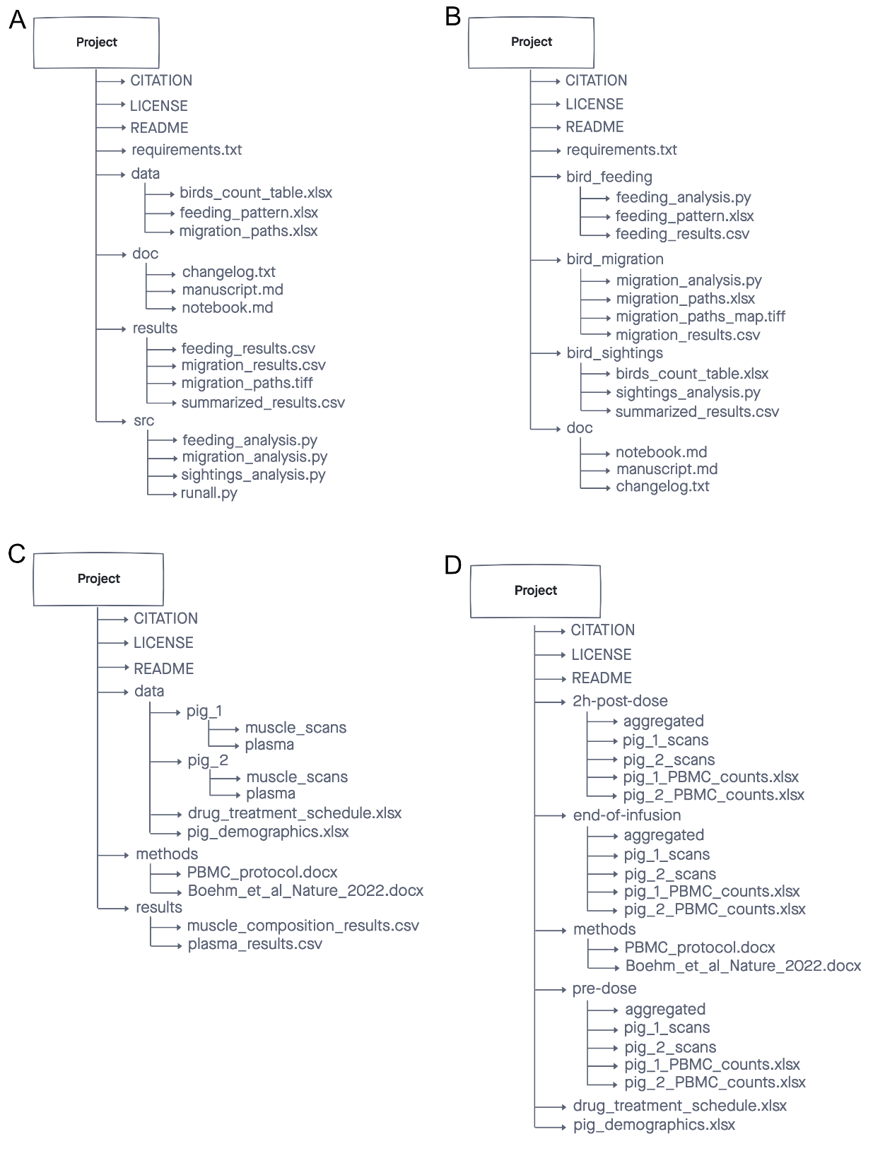 Figure credits: Ines Boehm
Reusable analysis
Figure 1
Select the notebook titled
‘student_notebook_light_conditions.ipynb’ as depicted below and click
‘Duplicate’. Confirm with Duplicate when you are asked if you are
certain that you want to duplicate the notebook.  Figure 1. Duplicate
a Jupyter notebook
Figure 1. Duplicate
a Jupyter notebook
Figure 2
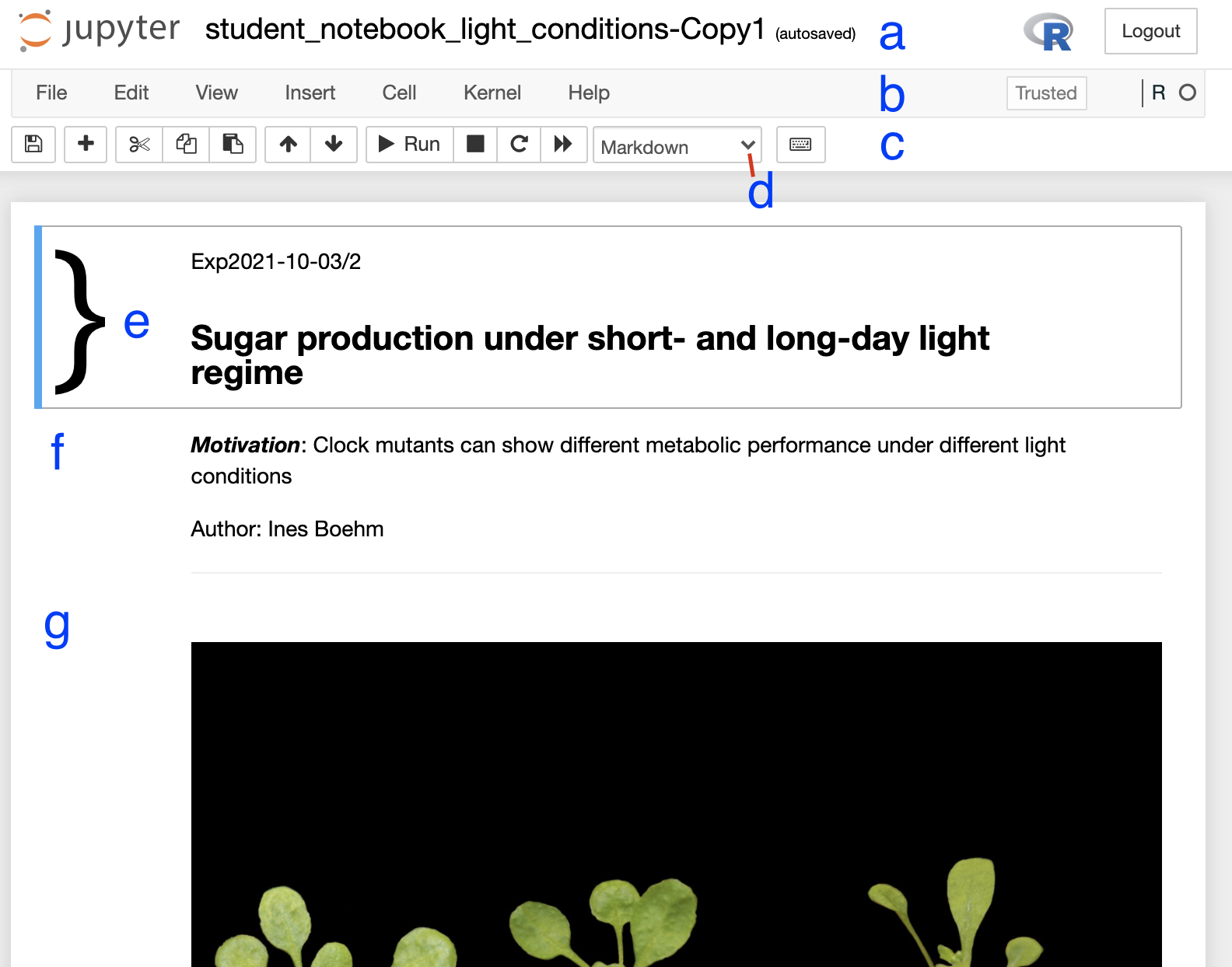
Figure 2. Anatomy of a Jupyter notebook: (a) depicts the name of the
notebook, (b, c) are toolbars, (c) contains the most commonly used
tools, (d) shows of what type - Markdown, Code etc… - the currently
selected cell is, and (e-g) are examples of cells, where (e) shows the
currently selected cell.
Figure 3
If you followed all steps correctly you should have reproduced the
table, a graph and statistical testing. Apart from the pre-filled
markdown text the rendered values of the code should look like this:
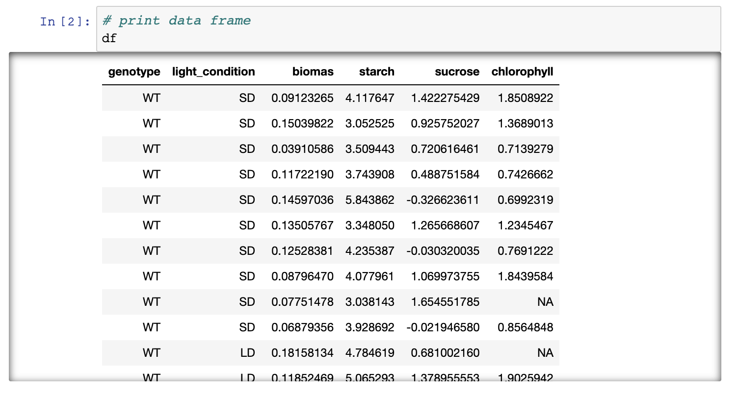
Figure 3. Rendering of data frame 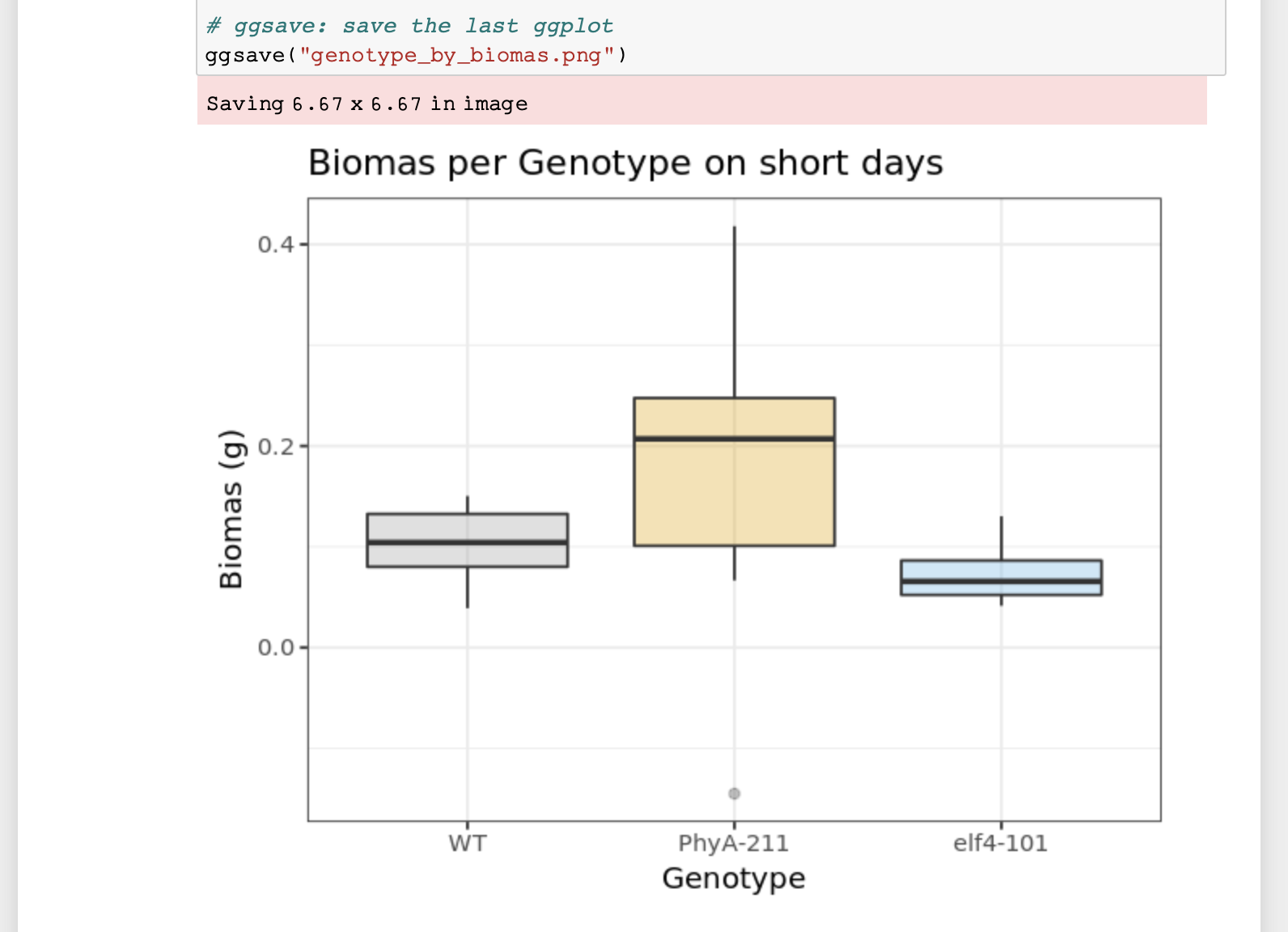
Figure 4. Rendering of plot
Public repositories
Figure 1
Journey to be FAIR
Figure 1
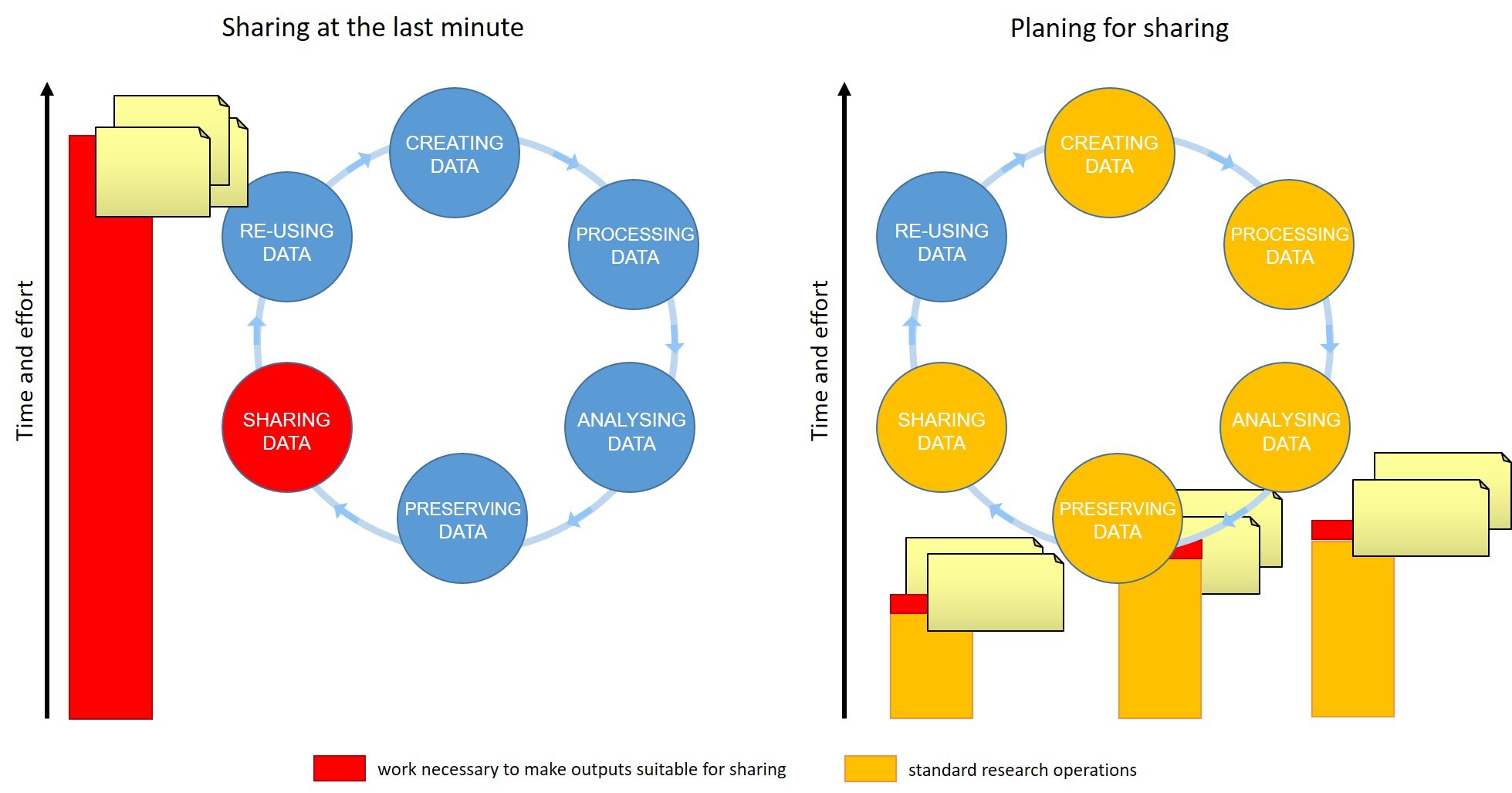 Figure credits:
Tomasz Zielinski and Andrés Romanowski
Figure credits:
Tomasz Zielinski and Andrés Romanowski