Bonus material

ML Pipeline Visualisation

---

To apply Deep Learning to a problem there are several steps we need to go through:

A visualisation of the Machine Learning Pipeline

Feel free to use this figure as png. The figure is contained in fig/graphviz/ of this repository. Use the Makefile there in order to reproduce it in different output formats.

Optional part - prediction uncertainty using Monte-Carlo Dropout

---

Depending on the data and the question asked, model predictions can be highly accuracte. Or, as in the present case, show a high degree of error. In both cases, however, it often is highly relevant to not get model predictions but also an estimate of how reliable those predictions are. The last years, this has been a very dynamic, rapidly growing area and there are many different ways to do uncertainty evaluation in deep learning. Here we want to present a very versatile and easy-to-implement method: Monte-Carlo Dropout (original reference: https://arxiv.org/abs/1506.02142).

The name of the technique refers to a very common regularization technique: Dropout. So let’s first introduce this:

Dropout: make it harder to memorize things

---

One of the most versatile regularization technique is dropout. Dropout essentially means that during each training cycle a random fraction of the dense layer nodes are turned off. This is described with the dropout rate between 0 and 1 which determines the fraction of nodes to silence at a time.

Dropout sketch

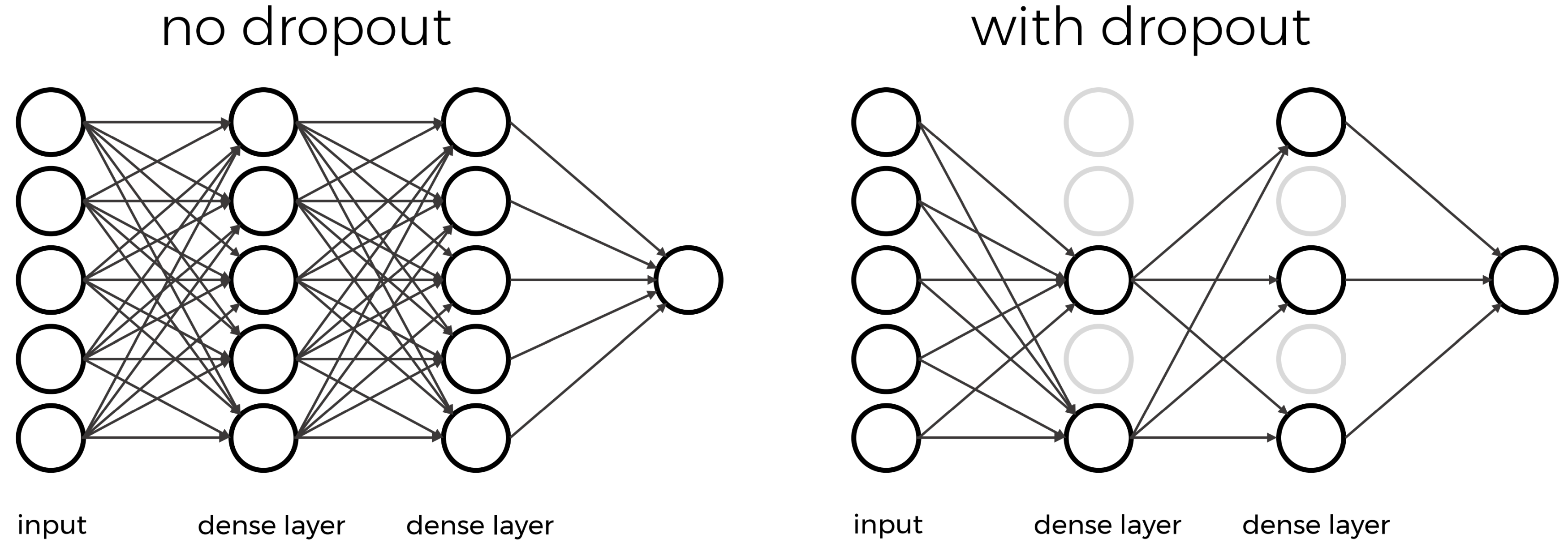
The intuition behind dropout is that it enforces redundancies in the network by constantly removing different elements of a network. The model can no longer rely on individual nodes and instead must create multiple “paths”. In addition, the model has to make predictions with much fewer nodes and weights (connections between the nodes). As a result, it becomes much harder for a network to memorize particular features. At first this might appear a quiet drastic approach which affects the network architecture strongly. In practice, however, dropout is computationally a very elegant solution which does not affet training speed. And it frequently works very well.

Important to note: Dropout layers will only randomly silence nodes during training! During a predictions step, all nodes remain active (dropout is off).

Let’s add dropout to our neural network which we will do by using keras Dropout layer (documentation & reference: https://keras.io/api/layers/regularization_layers/dropout/). One additional change that we will make here is to lower the learning rate because in the last training example the losses seemed to fluctuate a lot.

PYTHON

def create_nn(n_features, n_predictions):
    # Input layer
    layers_input = keras.layers.Input(shape=(n_features,), name='input')

    # Dense layers
    layers_dense = keras.layers.Dense(100, 'relu')(layers_input)
    layers_dense = keras.layers.Dropout(rate=0.2)(layers_dense)
    layers_dense = keras.layers.Dense(50, 'relu')(layers_dense)
    layers_dense = keras.layers.Dropout(rate=0.2)(layers_dense)

    # Output layer
    layers_output = keras.layers.Dense(n_predictions)(layers_dense)

    # Defining the model and compiling it
    return keras.Model(inputs=layers_input, outputs=layers_output, name="model_dropout")

model = create_nn(X_data.shape[1], 1)
model.compile(loss='mse', optimizer=keras.optimizers.Adam(1e-4), metrics=[keras.metrics.RootMeanSquaredError()])
model.summary()

OUTPUT

Model: "model_dropout"
_________________________________________________________________
Layer (type)                 Output Shape              Param #   
=================================================================
input (InputLayer)           [(None, 163)]             0         
_________________________________________________________________
dense_12 (Dense)             (None, 100)               16400     
_________________________________________________________________
dropout (Dropout)            (None, 100)               0         
_________________________________________________________________
dense_13 (Dense)             (None, 50)                5050      
_________________________________________________________________
dropout_1 (Dropout)          (None, 50)                0         
_________________________________________________________________
dense_14 (Dense)             (None, 1)                 51        
=================================================================
Total params: 21,501
Trainable params: 21,501
Non-trainable params: 0
_________________________________________________________________

Compared to the models above, this required little changes. We add two Dropout layers, one after each dense layer and specify the dropout rate. Here we use rate=0.2 which means that at any training step 20% of all nodes will be turned off. You can also see that Dropout layers do not add additional parameters. Now, let’s train our new model and plot the losses:

PYTHON

history = model.fit(X_train, y_train,
                    batch_size = 32,
                    epochs = 1000,
                    validation_data=(X_val, y_val),
                    callbacks=[earlystopper],
                    verbose = 2)

history_df = pd.DataFrame.from_dict(history.history)
sns.lineplot(data=history_df[['root_mean_squared_error', 'val_root_mean_squared_error']])
plt.xlabel("epochs")
plt.ylabel("RMSE")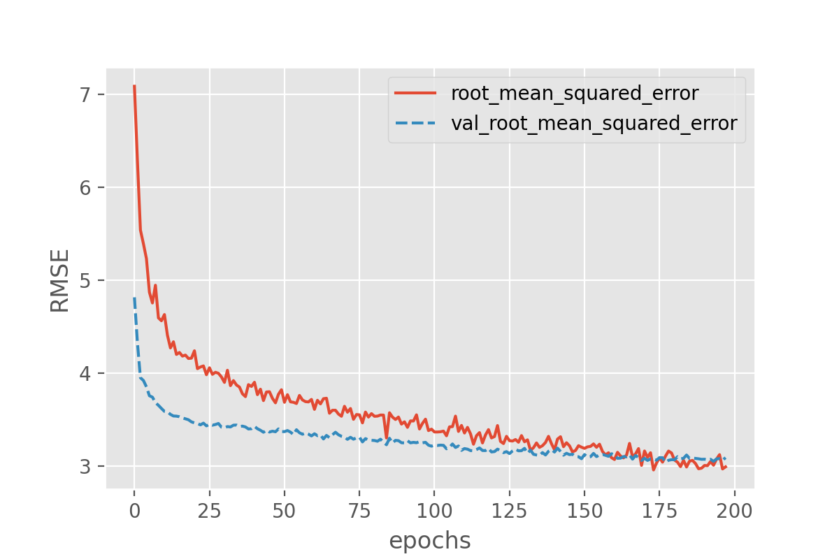

Output of plotting sample

In this setting overfitting seems to be pervented succesfully. The overall results though have not improved (at least not by much). Above we have used dropout to randomly turn off network nodes during training. When doing predictions, dropout is automatically deactivated and all nodes stay active. Each time you run the same input data through the same trained model, the prediciton will be exactly the same.

Monte-Carlo Dropout relies on a simply change: dropout will remain active during prediction! This means that each time a prediction step is done, the model will look differently because a fraction of all nodes will be turned off randomly. One can interpret all of those random variations as individual models. Monte-Carlo Dropout now makes use of this fact and collects many different predictions instead of only one. At the end this collection of predictions can be combined to a mean (or a median) prediction. And the variation of all predictions can tell something about the model’s uncertainty.

A simple (and a bit hacky) way to enforce dropout layers to remain active is to add training=True to the model:

PYTHON

def create_nn(n_features, n_predictions):
    # Input layer
    layers_input = keras.layers.Input(shape=(n_features,), name='input')

    # Dense layers
    layers_dense = keras.layers.BatchNormalization()(layers_input)
    layers_dense = keras.layers.Dense(100, 'relu')(layers_dense)
    layers_dense = keras.layers.Dropout(rate=0.2)(layers_dense, training=True)
    layers_dense = keras.layers.Dense(50, 'relu')(layers_dense)
    layers_dense = keras.layers.Dropout(rate=0.2)(layers_dense, training=True)

    # Output layer
    layers_output = keras.layers.Dense(n_predictions)(layers_dense)

    # Defining the model and compiling it
    return keras.Model(inputs=layers_input, outputs=layers_output, name="model_monte_carlo_dropout")

model = create_nn(X_data.shape[1], 1)
model.compile(loss='mse', optimizer=Adam(1e-4), metrics=[keras.metrics.RootMeanSquaredError()])

Model training remains entirely unchanged:

PYTHON

history = model.fit(X_train, y_train,
                    batch_size = 32,
                    epochs = 1000,
                    validation_data=(X_val, y_val),
                    callbacks=[earlystopper],
                    verbose = 2)

But when now doing predictions, things will look different. Let us do two predictions an compare the results.

PYTHON

y_test_predicted1 = model.predict(X_test)
y_test_predicted2 = model.predict(X_test)

y_test_predicted1[:10], y_test_predicted2[:10]

This should give two arrays with different float numbers.

We can now compute predictions for a larger ensemble, say 100 random variations of the same model:

from tqdm.notebook import tqdm  # optional: to add progress bar

n_ensemble = 100
y_test_predicted_ensemble = np.zeros((X_test.shape[0], n_ensemble))

for i in tqdm(range(n_ensemble)):  # or: for i in range(n_ensemble):
    y_test_predicted_ensemble[:, i] = model.predict(X_test)[:,0]

This will give an array of predictions, 100 different predictions for each datapoint in X_test. We can inspect an example distribution, for instance by plotting a histrogram:

PYTHON

plt.hist(y_test_predicted_ensemble[0,:], rwidth=0.9)
plt.xlabel("predicted sunshine hours")

Output of plotting sample

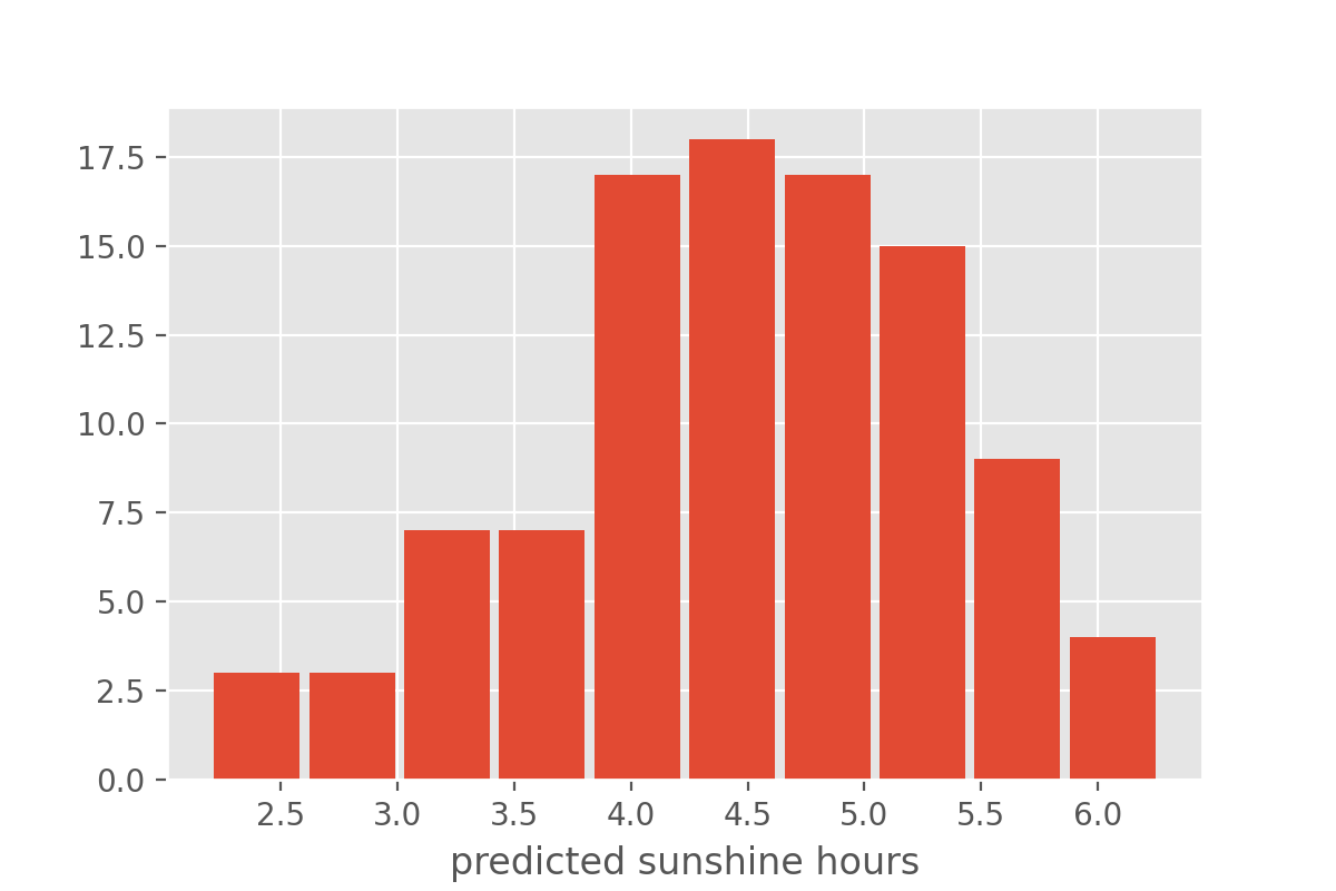
Instead of full distributions for every datapoint we might also just want to extract the mean and standard deviation.

y_test_predicted_mean = np.mean(y_test_predicted_ensemble, axis=1)
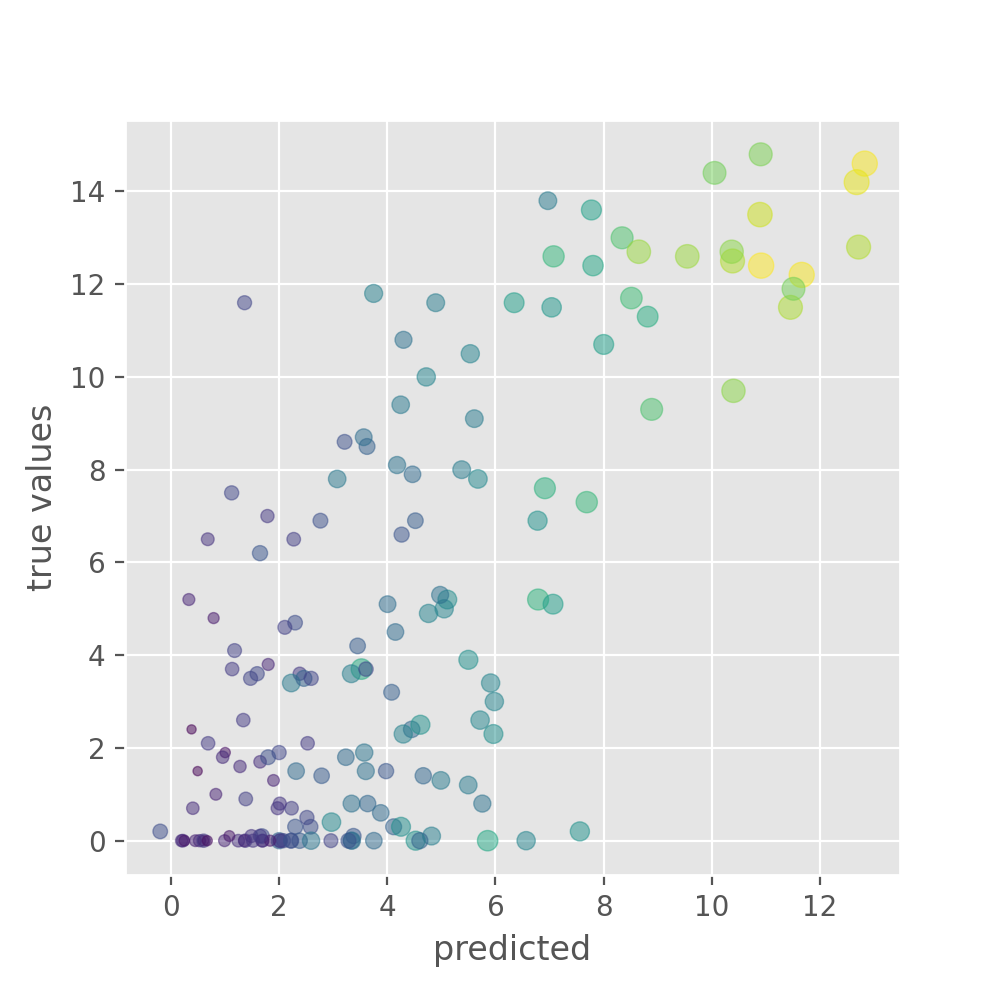
y_test_predicted_std = np.std(y_test_predicted_ensemble, axis=1)

This can then be plotted again as a scatter plot, but now with added information on the model uncertainty.

PYTHON

plt.figure(figsize=(5, 5), dpi=100)
plt.scatter(y_test_predicted_mean, y_test, s=40*y_test_predicted_std, 
            c=y_test_predicted_std, alpha=0.5)
plt.xlabel("predicted")
plt.ylabel("true values")

Output of plotting sample