Classification by a neural network using Keras
Last updated on 2025-01-21 | Edit this page
Overview
Questions
- How do I compose a neural network using Keras?
- How do I train this network on a dataset?
- How do I get insight into learning process?
- How do I measure the performance of the network?
Objectives
- Use the deep learning workflow to structure the notebook
- Explore the dataset using pandas and seaborn
- Identify the inputs and outputs of a deep neural network.
- Use one-hot encoding to prepare data for classification in Keras
- Describe a fully connected layer
- Implement a fully connected layer with Keras
- Use Keras to train a small fully connected network on prepared data
- Interpret the loss curve of the training process
- Use a confusion matrix to measure the trained networks’ performance on a test set
Introduction
In this episode we will learn how to create and train a neural network using Keras to solve a simple classification task.
The goal of this episode is to quickly get your hands dirty in actually defining and training a neural network, without going into depth of how neural networks work on a technical or mathematical level. We want you to go through the full deep learning workflow once before going into more details.
In fact, this is also what we would recommend you to do when working on real-world problems: First quickly build a working pipeline, while taking shortcuts. Then, slowly make the pipeline more advanced while you keep on evaluating the approach.
In episode 3 we will expand on the concepts that are lightly introduced in this episode. Some of these concepts include: how to monitor the training progress and how optimization works.
As a reminder below are the steps of the deep learning workflow:
- Formulate / Outline the problem
- Identify inputs and outputs
- Prepare data
- Choose a pretrained model or start building architecture from scratch
- Choose a loss function and optimizer
- Train the model
- Perform a Prediction/Classification
- Measure performance
- Refine the model
- Save model
In this episode we will focus on a minimal example for each of these steps, later episodes will build on this knowledge to go into greater depth for some or all of these steps.
GPU usage
For this lesson having a GPU (graphics processing unit) available is not needed. We specifically use very small toy problems so that you do not need one. However, Keras will use your GPU automatically when it is available. Using a GPU becomes necessary when tackling larger datasets or complex problems which require a more complex neural network.
1. Formulate/outline the problem: penguin classification
In this episode we will be using the penguin dataset. This is a dataset that was published in 2020 by Allison Horst and contains data on three different species of the penguins.
We will use the penguin dataset to train a neural network which can classify which species a penguin belongs to, based on their physical characteristics.
Goal
The goal is to predict a penguins’ species using the attributes available in this dataset.
The palmerpenguins data contains size measurements for
three penguin species observed on three islands in the Palmer
Archipelago, Antarctica. The physical attributes measured are flipper
length, beak length, beak width, body mass, and sex.

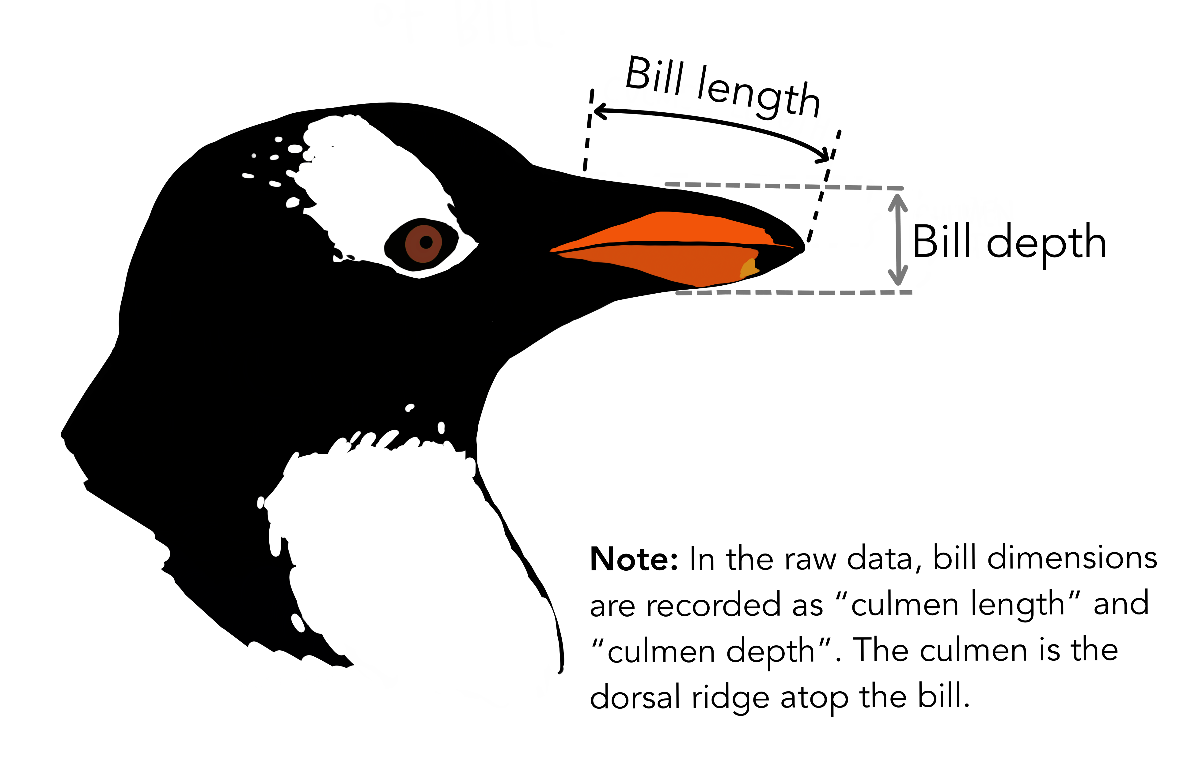
These data were collected from 2007 - 2009 by Dr. Kristen Gorman with the Palmer Station Long Term Ecological Research Program, part of the US Long Term Ecological Research Network. The data were imported directly from the Environmental Data Initiative (EDI) Data Portal, and are available for use by CC0 license (“No Rights Reserved”) in accordance with the Palmer Station Data Policy.
2. Identify inputs and outputs
To identify the inputs and outputs that we will use to design the neural network we need to familiarize ourselves with the dataset. This step is sometimes also called data exploration.
We will start by importing the Seaborn library that will help us get the dataset and visualize it. Seaborn is a powerful library with many visualizations. Keep in mind it requires the data to be in a pandas dataframe, luckily the datasets available in seaborn are already in a pandas dataframe.
We can load the penguin dataset using
This will give you a pandas dataframe which contains the penguin data.
Inspecting the data
Using the pandas head function gives us a quick look at
the data:
| species | island | bill_length_mm | bill_depth_mm | flipper_length_mm | body_mass_g | sex | |
|---|---|---|---|---|---|---|---|
| 0 | Adelie | Torgersen | 39.1 | 18.7 | 181.0 | 3750.0 | Male |
| 1 | Adelie | Torgersen | 39.5 | 17.4 | 186.0 | 3800.0 | Female |
| 2 | Adelie | Torgersen | 40.3 | 18.0 | 195.0 | 3250.0 | Female |
| 3 | Adelie | Torgersen | NaN | NaN | NaN | NaN | NaN |
| 4 | Adelie | Torgersen | 36.7 | 19.3 | 193.0 | 3450.0 | Female |
We can use all columns as features to predict the species of the
penguin, except for the species column itself.
Let’s look at the shape of the dataset:
There are 344 samples and 7 columns (plus the index column), so 6 features.
Visualization
Looking at numbers like this usually does not give a very good intuition about the data we are working with, so let us create a visualization.
Pair Plot
One nice visualization for datasets with relatively few attributes is
the Pair Plot. This can be created using sns.pairplot(...).
It shows a scatterplot of each attribute plotted against each of the
other attributes. By using the hue='species' setting for
the pairplot the graphs on the diagonal are layered kernel density
estimate plots for the different values of the species
column.
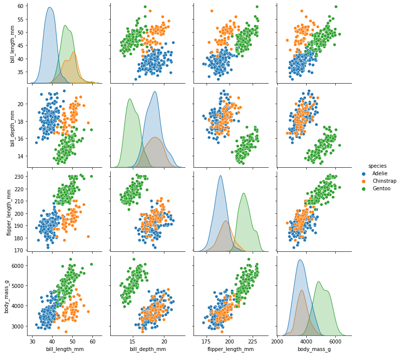
Pairplot
Take a look at the pairplot we created. Consider the following questions:
- Is there any class that is easily distinguishable from the others?
- Which combination of attributes shows the best separation for all 3 class labels at once?
- (optional) Create a similar pairplot, but with
hue="sex". Explain the patterns you see. Which combination of features distinguishes the two sexes best?
- The plots show that the green class, Gentoo is somewhat more easily distinguishable from the other two.
- The other two seem to be separable by a combination of bill length and bill depth (other combinations are also possible such as bill length and flipper length).
Answer to optional question:
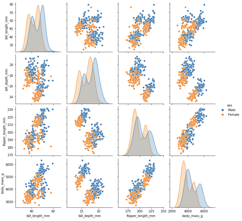
You see that for each species females have smaller bills and
flippers, as well as a smaller body mass. You would need a combination
of the species and the numerical features to successfully distinguish
males from females. The combination of bill_depth_mm and
body_mass_g gives the best separation.
Input and Output Selection
Now that we have familiarized ourselves with the dataset we can select the data attributes to use as input for the neural network and the target that we want to predict.
In the rest of this episode we will use the
bill_length_mm, bill_depth_mm,
flipper_length_mm, body_mass_g attributes. The
target for the classification task will be the species.
Data Exploration
Exploring the data is an important step to familiarize yourself with the problem and to help you determine the relevant inputs and outputs.
3. Prepare data
The input data and target data are not yet in a format that is suitable to use for training a neural network.
For now we will only use the numerical features
bill_length_mm, bill_depth_mm,
flipper_length_mm, body_mass_g only, so let’s
drop the categorical columns:
Clean missing values
During the exploration phase you may have noticed that some rows in
the dataset have missing (NaN) values, leaving such values in the input
data will ruin the training, so we need to deal with them. There are
many ways to deal with missing values, but for now we will just remove
the offending rows by adding a call to dropna():
Finally, we select only the features
Prepare target data for training
Second, the target data is also in a format that cannot be used in training. A neural network can only take numerical inputs and outputs, and learns by calculating how “far away” the species predicted by the neural network is from the true species.
When the target is a string category column as we have here, we need to transform this column into a numerical format first. Again, there are many ways to do this. We will be using the one-hot encoding. This encoding creates multiple columns, as many as there are unique values, and puts a 1 in the column with the corresponding correct class, and 0’s in the other columns. For instance, for a penguin of the Adelie species the one-hot encoding would be 1 0 0.
Fortunately, Pandas is able to generate this encoding for us.
PYTHON
import pandas as pd

target = pd.get_dummies(penguins_filtered['species'])
target.head() # print out the top 5 to see what it looks like.
One-hot encoding
How many output neurons will our network have now that we one-hot encoded the target class?
- A: 1
- B: 2
- C: 3
C: 3, one for each output variable class
Split data into training and test set
Finally, we will split the dataset into a training set and a test set. As the names imply we will use the training set to train the neural network, while the test set is kept separate. We will use the test set to assess the performance of the trained neural network on unseen samples. In many cases a validation set is also kept separate from the training and test sets (i.e. the dataset is split into 3 parts). This validation set is then used to select the values of the parameters of the neural network and the training methods. For this episode we will keep it at just a training and test set however.
To split the cleaned dataset into a training and test set we will use
a very convenient function from sklearn called
train_test_split.
This function takes a number of parameters which are extensively explained in the scikit-learn documentation :
- The first two parameters are the dataset (in our case
features) and the corresponding targets (i.e. defined as target). - Next is the named parameter
test_sizethis is the fraction of the dataset that is used for testing, in this case0.2means 20% of the data will be used for testing. -
random_statecontrols the shuffling of the dataset, setting this value will reproduce the same results (assuming you give the same integer) every time it is called. -
shufflewhich can be eitherTrueorFalse, it controls whether the order of the rows of the dataset is shuffled before splitting. It defaults toTrue. -
stratifyis a more advanced parameter that controls how the split is done. By setting it totargetthe train and test sets the function will return will have roughly the same proportions (with regards to the number of penguins of a certain species) as the dataset.
PYTHON
from sklearn.model_selection import train_test_split

X_train, X_test, y_train, y_test = train_test_split(features, target, test_size=0.2, random_state=0, shuffle=True, stratify=target)
Importance of using the same train-test split
By setting random_state=0 we ensure that everyone has
the same train-test split. When doing machine learning and deep learning
it is crucial that you use the same train and test dataset for different
experiments. Comparing evaluation metrics between experiments run on
different data splits is meaningless, because the accuracy of a model
depends on the data used to train and test it.
4. Build an architecture from scratch or choose a pretrained model
Keras for neural networks
Keras is a machine learning framework with ease of use as one of its
main features. It is part of the tensorflow python package and can be
imported using from tensorflow import keras.
Keras includes functions, classes and definitions to define deep learning models, cost functions and optimizers (optimizers are used to train a model).
Before we move on to the next section of the workflow we need to make sure we have Keras imported. We do this as follows:
For this episode it is useful if everyone gets the same results from their training. Keras uses a random number generator at certain points during its execution. Therefore we will need to set two random seeds, one for numpy and one for tensorflow:
When to use random seeds?
We use a random seed here to ensure that we get the same results every time we run this code. This makes our results reproducible and allows us to better compare results between different experiments.
Please note that even though you have selected a random seed, this seed is used to generate a different random number every time you execute a Jupyter cell. So, to get truly replicable deep learning pipelines you need to run the notebook from start to end in one go.
Build a neural network from scratch
We will now build a simple neural network from scratch using Keras.
With Keras you compose a neural network by creating layers and
linking them together. For now we will only use one type of layer called
a fully connected or Dense layer. In Keras this is defined by the
keras.layers.Dense class.
A dense layer has a number of neurons, which is a parameter you can choose when you create the layer. When connecting the layer to its input and output layers every neuron in the dense layer gets an edge (i.e. connection) to all of the input neurons and all of the output neurons. The hidden layer in the image in the introduction of this episode is a Dense layer.
The input in Keras also gets special treatment, Keras automatically
calculates the number of inputs and outputs a layer needs and therefore
how many edges need to be created. This means we need to inform Keras
how big our input is going to be. We do this by instantiating a
keras.Input class and tell it how big our input is, thus
the number of columns it contains.
We store a reference to this input class in a variable so we can pass it to the creation of our hidden layer. Creating the hidden layer can then be done as follows:
The instantiation here has 2 parameters and a seemingly strange
combination of parentheses, so let us take a closer look. The first
parameter 10 is the number of neurons we want in this
layer, this is one of the hyperparameters of our system and needs to be
chosen carefully. We will get back to this in the section on refining
the model.
The second parameter is the activation function to use. We choose
relu which returns 0 for inputs that are 0 and below and
the identity function (returning the same value) for inputs above 0.
This is a commonly used activation function in deep neural networks that
is proven to work well.
Next we see an extra set of parenthenses with inputs in them. This means that after creating an instance of the Dense layer we call it as if it was a function. This tells the Dense layer to connect the layer passed as a parameter, in this case the inputs.
Finally we store a reference in the hidden_layer
variable so we can pass it to the output layer in a minute.
Now we create another layer that will be our output layer. Again we use a Dense layer and so the call is very similar to the previous one.
Because we chose the one-hot encoding, we use three neurons for the output layer.
The softmax activation ensures that the three output
neurons produce values in the range (0, 1) and they sum to 1. We can
interpret this as a kind of ‘probability’ that the sample belongs to a
certain species.
Now that we have defined the layers of our neural network we can combine them into a Keras model which facilitates training the network.
The model summary here can show you some information about the neural network we have defined.
Trainable and non-trainable parameters
Keras distinguishes between two types of weights, namely:
trainable parameters: these are weights of the neurons that are modified when we train the model in order to minimize our loss function (we will learn about loss functions shortly!).
non-trainable parameters: these are weights of the neurons that are not changed when we train the model. These could be for many reasons - using a pre-trained model, choice of a particular filter for a convolutional neural network, and statistical weights for batch normalization are some examples.
If these reasons are not clear right away, don’t worry! In later episodes of this course, we will touch upon a couple of these concepts.
Create the neural network
With the code snippets above, we defined a Keras model with 1 hidden layer with 10 neurons and an output layer with 3 neurons.
- How many parameters does the resulting model have?
- What happens to the number of parameters if we increase or decrease the number of neurons in the hidden layer?
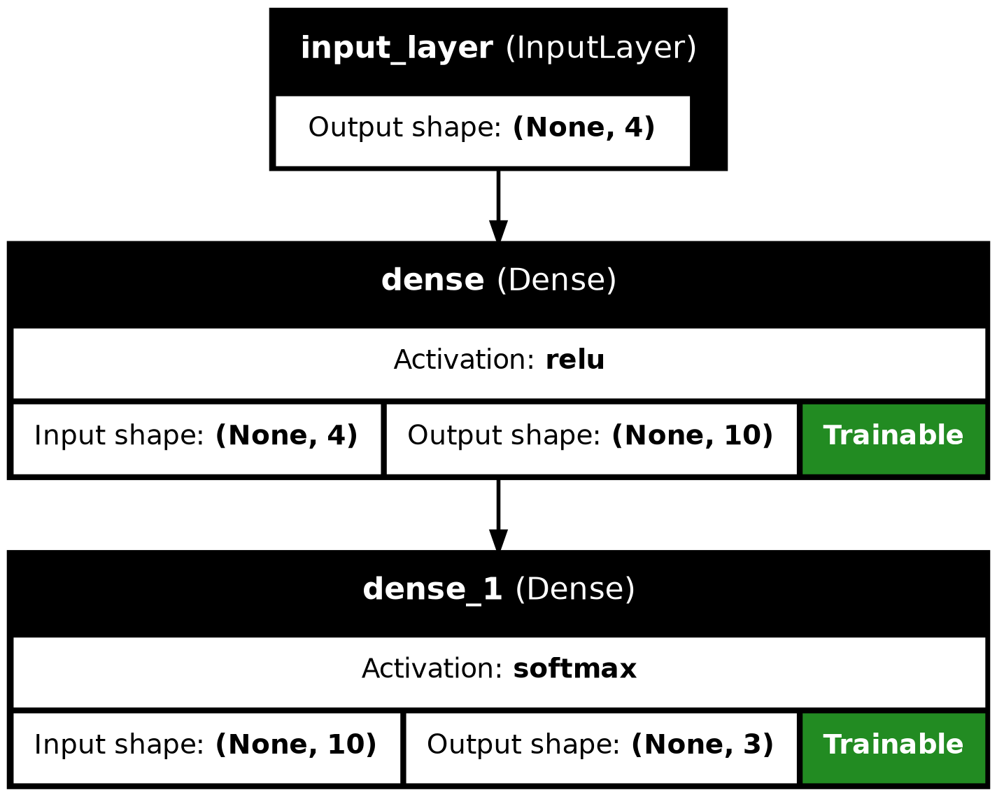
(optional) Visualizing the model
Optionally, you can also visualize the same information as
model.summary() in graph form. This step requires the
command-line tool dot from Graphviz installed, you
installed it by following the setup instructions. You can check that the
installation was successful by executing dot -V in the
command line. You should get something as follows:
- (optional) Provided you have
dotinstalled, execute theplot_modelfunction as shown below.
(optional) Keras Sequential vs Functional API
So far we have used the Functional API of Keras. You can also implement neural networks using the Sequential model. As you can read in the documentation, the Sequential model is appropriate for a plain stack of layers where each layer has exactly one input tensor and one output tensor.
- (optional) Use the Sequential model to implement the same network
Have a look at the output of model.summary():
OUTPUT
Model: "functional"

┏━━━━━━━━━━━━━━━━━━━━━━━━━━━━┳━━━━━━━━━━━━━━━━┳━━━━━━━━━━━━┓
┃ Layer (type)               ┃ Output Shape   ┃    Param # ┃
┡━━━━━━━━━━━━━━━━━━━━━━━━━━━━╇━━━━━━━━━━━━━━━━╇━━━━━━━━━━━━┩
│ input_layer (InputLayer)   │ (None, 4)      │          0 │
├────────────────────────────┼────────────────┼────────────┤
│ dense (Dense)              │ (None, 10)     │         50 │
├────────────────────────────┼────────────────┼────────────┤
│ dense_1 (Dense)            │ (None, 3)      │         33 │
└────────────────────────────┴────────────────┴────────────┘

 Total params: 83 (332.00 B)

 Trainable params: 83 (332.00 B)

 Non-trainable params: 0 (0.00 B)
The model has 83 trainable parameters. Each of the 10 neurons in the
in the dense hidden layer is connected to each of the 4
inputs in the input layer resulting in 40 weights that can be trained.
The 10 neurons in the hidden layer are also connected to each of the 3
outputs in the dense_1 output layer, resulting in a further
30 weights that can be trained. By default Dense layers in
Keras also contain 1 bias term for each neuron, resulting in a further
10 bias values for the hidden layer and 3 bias terms for the output
layer. 40+30+10+3=83 trainable parameters.
The value (332.00 B) next to it describes the memory
footprint for model weights and this depends on their data type. Take a
look at what model.dtype is.
OUTPUT
float32The model weights are represented using float32 data
type, which consumes 32 bits or 4 bytes for each weight. We have 83
parameters, and therefore in total, the model requires
83*4=332 bytes of memory to load into the computer’s
memory.
If you increase the number of neurons in the hidden layer the number of trainable parameters in both the hidden and output layer increases or decreases in accordance with the number of neurons added. Each extra neuron has 4 weights connected to the input layer, 1 bias term, and 3 weights connected to the output layer. So in total 8 extra parameters.
The name in quotes within the string
Model: "functional" may be different in your view; this
detail is not important.
(optional) Visualizing the model
- Upon executing the
plot_modelfunction, you should see the following image.
(optional) Keras Sequential vs Functional API
- This implements the same model using the Sequential API:
PYTHON
model = keras.Sequential(
    [
        keras.Input(shape=(X_train.shape[1],)),
        keras.layers.Dense(10, activation="relu"),
        keras.layers.Dense(3, activation="softmax"),
    ]
)
We will use the Functional API for the remainder of this course, since it is more flexible and more explicit.
How to choose an architecture?
Even for this small neural network, we had to make a choice on the number of hidden neurons. Other choices to be made are the number of layers and type of layers (as we will see later). You might wonder how you should make these architectural choices. Unfortunately, there are no clear rules to follow here, and it often boils down to a lot of trial and error. However, it is recommended to look what others have done with similar datasets and problems. Another best practice is to start with a relatively simple architecture. Once running start to add layers and tweak the network to see if performance increases.
Choose a pretrained model
If your data and problem is very similar to what others have done, you can often use a pretrained network. Even if your problem is different, but the data type is common (for example images), you can use a pretrained network and finetune it for your problem. A large number of openly available pretrained networks can be found on Hugging Face (especially LLMs), MONAI (medical imaging), the Model Zoo, pytorch hub or tensorflow hub.
5. Choose a loss function and optimizer
We have now designed a neural network that in theory we should be able to train to classify Penguins. However, we first need to select an appropriate loss function that we will use during training. This loss function tells the training algorithm how wrong, or how ‘far away’ from the true value the predicted value is.
For the one-hot encoding that we selected earlier a suitable loss
function is the Categorical Crossentropy loss. In Keras this is
implemented in the keras.losses.CategoricalCrossentropy
class. This loss function works well in combination with the
softmax activation function we chose earlier. The
Categorical Crossentropy works by comparing the probabilities that the
neural network predicts with ‘true’ probabilities that we generated
using the one-hot encoding. This is a measure for how close the
distribution of the three neural network outputs corresponds to the
distribution of the three values in the one-hot encoding. It is lower if
the distributions are more similar.
For more information on the available loss functions in Keras you can check the documentation.
Next we need to choose which optimizer to use and, if this optimizer has parameters, what values to use for those. Furthermore, we need to specify how many times to show the training samples to the optimizer.
Once more, Keras gives us plenty of choices all of which have their own pros and cons, but for now let us go with the widely used Adam optimizer. Adam has a number of parameters, but the default values work well for most problems. So we will use it with its default parameters.
Combining this with the loss function we decided on earlier we can
now compile the model using model.compile. Compiling the
model prepares it to start the training.
6. Train model
We are now ready to train the model.
Training the model is done using the fit method, it
takes the input data and target data as inputs and it has several other
parameters for certain options of the training. Here we only set a
different number of epochs. One training epoch means that
every sample in the training data has been shown to the neural network
and used to update its parameters.
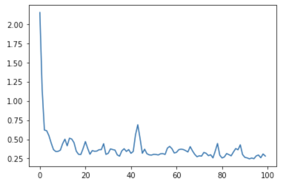
The fit method returns a history object that has a history attribute with the training loss and potentially other metrics per training epoch. It can be very insightful to plot the training loss to see how the training progresses. Using seaborn we can do this as follows:
I get a different plot
It could be that you get a different plot than the one shown here.
This could be because of a different random initialization of the model
or a different split of the data. This difference can be avoided by
setting random_state and random seed in the same way like
we discussed in When to use random
seeds?.
This plot can be used to identify whether the training is well configured or whether there are problems that need to be addressed.
The Training Curve
Looking at the training curve we have just made.
- How does the training progress?
- Does the training loss increase or decrease?
- Does it change quickly or slowly?
- Does the graph look very jittery?
- Do you think the resulting trained network will work well on the test set?
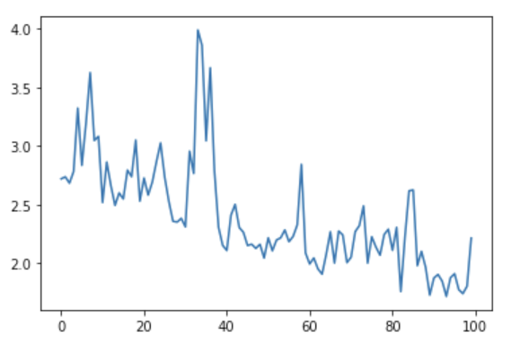
When the training process does not go well:
- (optional) Something went wrong here during training. What could be
the problem, and how do you see that in the training curve? Also compare
the range on the y-axis with the previous training curve.
- The training loss decreases quickly. It drops in a smooth line with little jitter. This is ideal for a training curve.
- The results of the training give very little information on its performance on a test set. You should be careful not to use it as an indication of a well trained network.
- (optional) The loss does not go down at all, or only very slightly. This means that the model is not learning anything. It could be that something went wrong in the data preparation (for example the labels are not attached to the right features). In addition, the graph is very jittery. This means that for every update step, the weights in the network are updated in such a way that the loss sometimes increases a lot and sometimes decreases a lot. This could indicate that the weights are updated too much at every learning step and you need a smaller learning rate (we will go into more details on this in the next episode). Or there is a high variation in the data, leading the optimizer to change the weights in different directions at every learning step. This could be addressed by presenting more data at every learning step (or in other words increasing the batch size). In this case the graph was created by training on nonsense data, so this a training curve for a problem where nothing can be learned really.
We will take a closer look at training curves in the next episode. Some of the concepts touched upon here will also be further explained there.
7. Perform a prediction/classification
Now that we have a trained neural network, we can use it to predict
new samples of penguin using the predict function.
We will use the neural network to predict the species of the test set
using the predict function. We will be using this
prediction in the next step to measure the performance of our trained
network. This will return a numpy matrix, which we convert
to a pandas dataframe to easily see the labels.
PYTHON
y_pred = model.predict(X_test)
prediction = pd.DataFrame(y_pred, columns=target.columns)
prediction| 0 | 0.304484 | 0.192893 | 0.502623 |
| 1 | 0.527107 | 0.095888 | 0.377005 |
| 2 | 0.373989 | 0.195604 | 0.430406 |
| 3 | 0.493643 | 0.154104 | 0.352253 |
| 4 | 0.309051 | 0.308646 | 0.382303 |
| … | … | … | … |
| 64 | 0.406074 | 0.191430 | 0.402496 |
| 65 | 0.645621 | 0.077174 | 0.277204 |
| 66 | 0.356284 | 0.185958 | 0.457758 |
| 67 | 0.393868 | 0.159575 | 0.446557 |
| 68 | 0.509837 | 0.144219 | 0.345943 |
Remember that the output of the network uses the softmax
activation function and has three outputs, one for each species. This
dataframe shows this nicely.
We now need to transform this output to one penguin species per
sample. We can do this by looking for the index of highest valued output
and converting that to the corresponding species. Pandas dataframes have
the idxmax function, which will do exactly that.
OUTPUT
0     Gentoo
1     Adelie
2     Gentoo
3     Adelie
4     Gentoo
      ...
64    Adelie
65    Adelie
66    Gentoo
67    Gentoo
68    Adelie
Length: 69, dtype: object
8. Measuring performance
Now that we have a trained neural network it is important to assess how well it performs. We want to know how well it will perform in a realistic prediction scenario, measuring performance will also come back when refining the model.
We have created a test set (i.e. y_test) during the data preparation stage which we will use now to create a confusion matrix.
Confusion matrix
With the predicted species we can now create a confusion matrix and display it using seaborn.
A confusion matrix is an N x N matrix used for
evaluating the performance of a classification model, where
N is the number of target classes. The matrix compares the
actual target values with those predicted from the classification model,
which gives a holistic view of how well the classification model is
performing.
To create a confusion matrix we will use another convenience function
from sklearn called confusion_matrix. This function takes
as a first parameter the true labels of the test set. We can get these
by using the idxmax method on the y_test dataframe. The
second parameter is the predicted labels which we did above.
PYTHON
from sklearn.metrics import confusion_matrix

true_species = y_test.idxmax(axis="columns")

matrix = confusion_matrix(true_species, predicted_species)
print(matrix)
OUTPUT
[[22  0  8]
 [ 5  0  9]
 [ 6  0 19]]
Unfortunately, this matrix is not immediately understandable. Its not clear which column and which row corresponds to which species. So let’s convert it to a Pandas Dataframe with its index and columns set to the species as follows:
PYTHON
# Convert to a pandas dataframe
confusion_df = pd.DataFrame(matrix, index=y_test.columns.values, columns=y_test.columns.values)

# Set the names of the x and y axis, this helps with the readability of the heatmap.
confusion_df.index.name = 'True Label'
confusion_df.columns.name = 'Predicted Label'
confusion_df.head()
We can then use the heatmap function from seaborn to
create a nice visualization of the confusion matrix. The
annot=True parameter here will put the numbers from the
confusion matrix in the heatmap.
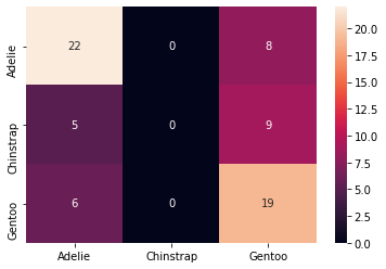
Here are more explanations of this confusion matrix and the classification model. - The first row: There are 30 Adelie penguins in the test data, with 22 identified as Adelie (valid), 8 being identified as Gentoo (invalid), and no Adelie is identified as Chinstrap. - The second row: There are 14 Chinstrap pengunis in the test data, with 5 identified as Adelie (invalid), none are correctly recognized as Chinstrap, and 9 Chinstraps are identified as Gentoo (invalid). - The third row: There are 25 Gentoo penguins in the test data, with 6 identified as Adelie (invalid), none being recognized as Chinstrap (invalid), and 19 Gentoos are identified as Gentoo (valid).
Confusion Matrix
Measure the performance of the neural network you trained and visualize a confusion matrix.
- Did the neural network perform well on the test set?
- Did you expect this from the training loss you saw?
- What could we do to improve the performance?
The confusion matrix shows that the predictions for Adelie and Gentoo are decent, but could be improved. However, Chinstrap is not predicted ever.
If we go back to the Pair Plot in the Visualization section above, we can figure out that the biggest challenge is distinguishing the Chinstrap penguins from the marginal distributions of the four features (bill length, bill depth, flipper length, and body mass). That means that there is no single variable that separates Chinstrap penguins from all other species. Only the combination of bill length and bill depth gives a good separation of Chinstrap from Adelie and Gentoo penguins.
The training loss was very low, so the low accuracy on the test set may be surprising. But this illustrates very well why a test set is important to give a realistic evaluation when training neural networks (or other machine learning classifiers).
We can try many things to improve the performance from here. One of the first things we can try is to balance the dataset better.
Furthermore, the constructed neural network has a limited number of parameters. A practical workaround is to increase the number of dense layers and also the number of neurons in each dense layers.
In addition, adjusting the learning rate can also help achieving a high score for the prediction. You will get more info in the Advanced layer types episode.
Note that the outcome you have might be slightly different from what is shown in this tutorial.
9. Refine the model
As we discussed before the design and training of a neural network comes with many hyperparameter and model architecture choices. We will go into more depth of these choices in later episodes. For now it is important to realize that the parameters we chose were somewhat arbitrary and more careful consideration needs to be taken to pick hyperparameter values.
10. Share model
It is very useful to be able to use the trained neural network at a
later stage without having to retrain it. This can be done by using the
save method of the model. It takes a string as a parameter
which is the path of a directory where the model is stored.
This saved model can be loaded again by using the
load_model method as follows:
This loaded model can be used as before to predict.
PYTHON
# use the pretrained model here
y_pretrained_pred = pretrained_model.predict(X_test)
pretrained_prediction = pd.DataFrame(y_pretrained_pred, columns=target.columns.values)

# idxmax will select the column for each row with the highest value
pretrained_predicted_species = pretrained_prediction.idxmax(axis="columns")
print(pretrained_predicted_species)
OUTPUT
0     Adelie
1     Gentoo
2     Adelie
3     Gentoo
4     Gentoo
      ...
64    Gentoo
65    Gentoo
66    Adelie
67    Adelie
68    Gentoo
Length: 69, dtype: object
Key Points
- The deep learning workflow is a useful tool to structure your approach, it helps to make sure you do not forget any important steps.
- Exploring the data is an important step to familiarize yourself with the problem and to help you determine the relavent inputs and outputs.
- One-hot encoding is a preprocessing step to prepare labels for classification in Keras.
- A fully connected layer is a layer which has connections to all neurons in the previous and subsequent layers.
- keras.layers.Dense is an implementation of a fully connected layer, you can set the number of neurons in the layer and the activation function used.
- To train a neural network with Keras we need to first define the network using layers and the Model class. Then we can train it using the model.fit function.
- Plotting the loss curve can be used to identify and troubleshoot the training process.
- The loss curve on the training set does not provide any information on how well a network performs in a real setting.
- Creating a confusion matrix with results from a test set gives better insight into the network’s performance.
