sMRI Acquisition and Modalities
Last updated on 2025-02-26 | Edit this page
Overview
Questions
- How is a structural MR image acquired?
- What anatomical features do different modalities capture?
Objectives
- Visualize and understand differences in T1,T2,PD/FLAIR weighted images.
You Are Here!
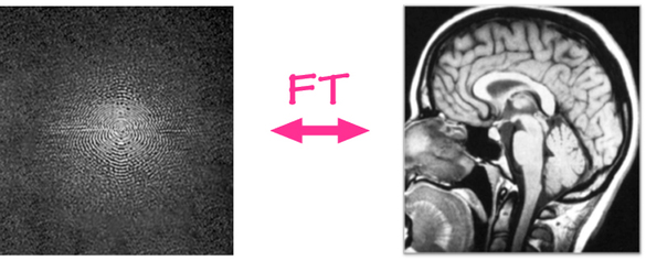
Image acquisition
The acquisition starts with application of strong magnetic field B0 (e.g. 1.5 or 3.0 Tesla > 10000x earth’s magnetic field) which forces the hydrogen nuclei of the abundant water molecules in soft tissues in the body to align with the field. You can think of hydrogen nuclei as tiny magnets of their own.
Then the scanner applies a radio-frequency (RF) (i.e. excitation) pulse which tilts these nuclei from their alignment along B0. The nuclei then precess back to the alignment. The precessing nuclei emit a signal, which is registered by the receiver coils in the scanner.
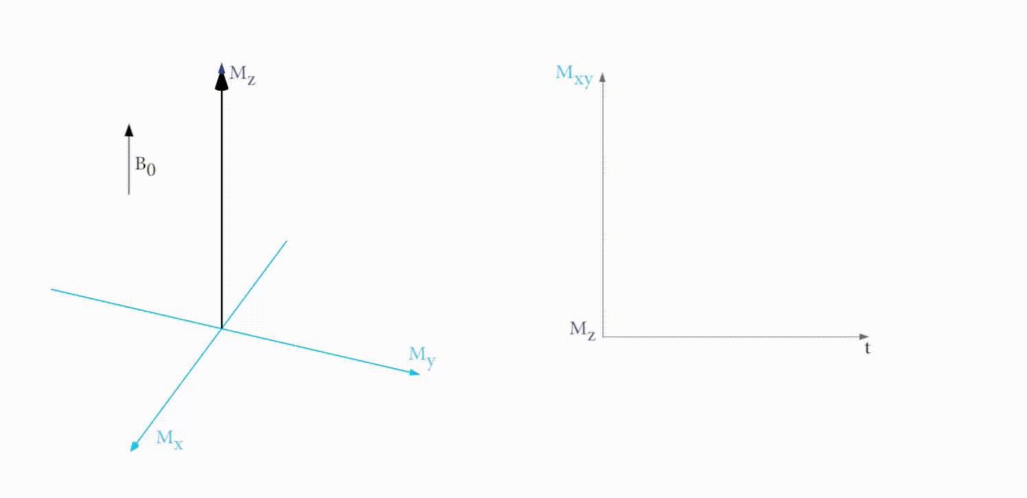
This signal has two components: 1) Longitudinal (z-axis along the scanner’s magnetic field) and 2) Transverse (xy-plane orthogonal to the scanner’s magnetic field).
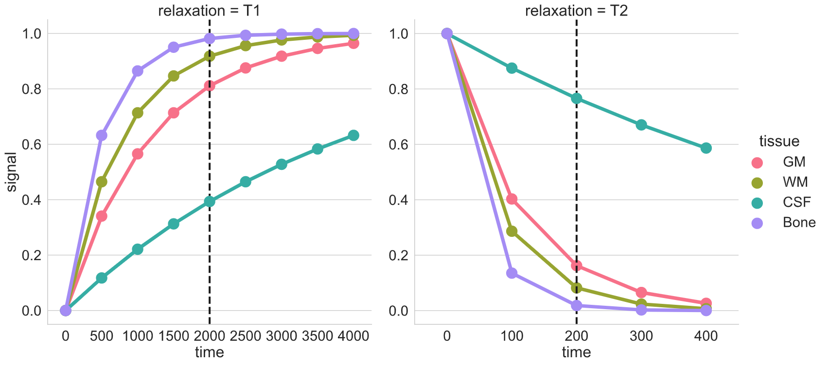
Initially the longitudinal signal is weak as most nuclei are tilted away from the z-axis. However this signal grows as nuclei realign. The time constant that dictates the speed of re-alignment is denoted by T1.
Initially the transverse signal is strong as most nuclei are in phase coherence. The signal decays as the nuclei dephase as they realign. This decay is denoted by the T2 time constant.
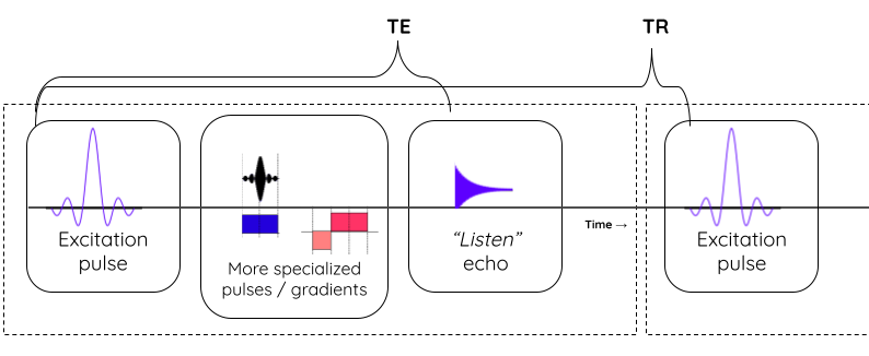
The tissue specific differences in T1 and T2 relaxation times is what enables us to see anatomy from image contrast. The final image contrast depends on when you listen to the signal (design parameter: echo time (TE)) and how fast you repeat the tilt-relax process i.e. RF pulse frequency (design parameter: repetition time (TR)).
T1 and T2 relaxation
Here we see signal from two different tissues as the nuclei are tilted and realigned. The figure on the left shows a single nucleus (i.e. tiny magnet) being tilted away and then precessing back to the the initial alighment along B0. The figure on the right shows the corresponding registered T1 and T2 signal profiles for two different “tissues”. The difference in their signal intensities results in the image contrast.
Brain tissue comparison
The dotted-black line represents the epoch when you “listen” to the signal (i.e. echo time or TE).
 )
)
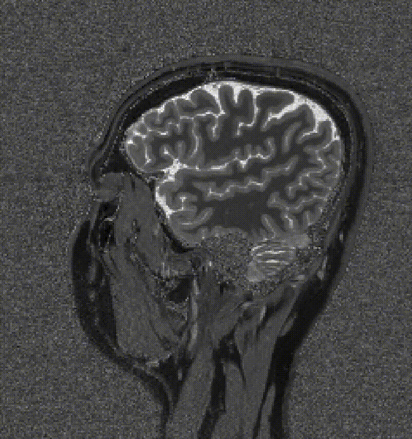
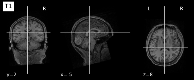
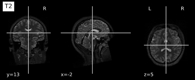
T1w, T2w, and PD acquisition
| TE short | TE long (~ T2 of tissue of interest) | |
|---|---|---|
| TR short (~ T1 of tissue of interest) | T1w | - |
| TR long | Proton Density (PD) | T2w |
Note: More recently, the FLAIR (Fluid Attenuated Inversion Recovery) sequence has replaced the PD image. FLAIR images are T2-weighted with the CSF signal suppressed.
pulse sequence parameters and image contrast
What are the two basic pulse sequence parameters that impact T1w and T2w image contrasts? Which one is larger?
Repetition time (TR) and echo time (TE) are the two pulse sequence parameters that dictate the T1w and T2w image contrasts. TR > TE.
T1 and T2 relaxation times for various tissues
| T1 (ms) | T2 (ms) | |
|---|---|---|
| Bones | 500 | 50 |
| CSF | 4000 | 500 |
| Grey Matter | 1300 | 110 |
| White Matter | 800 | 80 |
Tissue type and image contrast
In the T1w image, which one is brighter: White matter, Grey Matter, or CSF?
White Matter (i.e. axonal tracts)
Applications per modality
| Modality | Contrast Characteristics | Use Cases |
|---|---|---|
| T1w | Cerebrospinal fluid is dark | Quantifying anatomy e.g. measure structural volumes |
| T2w | CSF is light, but white matter is darker than with T1 | Identify pathologies related to lesions and tumors |
| PD | CSF is bright. Gray matter is brighter than white matter | Identify demyelination |
| FLAIR | Similar to T2 with the CSF signal suppressed | Identify demyelination |
Image acquisition process and parameters
What do we want?
- High image contrast
- High spatial resolution
- Low scan time!
What can we control?
Magnetic strengths 1.5T vs 3T vs 7T
- Higher magnetic strength –> better spatial resolution, better SNR (S ∝ B0^2); but more susceptible to certain artifacts.
MR sequences (i.e. timings of “excitation pulse”, “gradients”, and “echo acquisition” )
- Spin echo: Slower but better contrast to noise ratio (CNR)
- Gradient echo: Quicker but more susceptible to noise
e.g. MPRAGE: Magnetization Prepared - RApid Gradient Echo (Commonly used in neuroimaging)
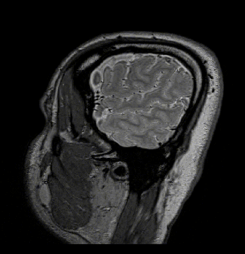
| MP-RAGE | MP2-RAGE |
|---|---|
 |
 |
Interacting with images (see this notebook for detailed example.)
PYTHON
local_data_dir = '../local_data/1_sMRI_modalities/'
T1_filename = local_data_dir + 'craving_sub-SAXSISO01b_T1w.nii.gz'
T2_filename = local_data_dir +'craving_sub-SAXSISO01b_T2w.nii.gz'
T1_img = nib.load(T1_filename)
T2_img = nib.load(T2_filename)
# grab data array
T1_data = T1_img.get_fdata()
T2_data = T2_img.get_fdata()
# plot
plotting.plot_anat(T1_filename, title="T1", vmax=500)
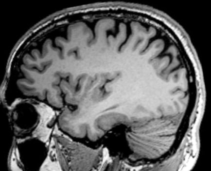
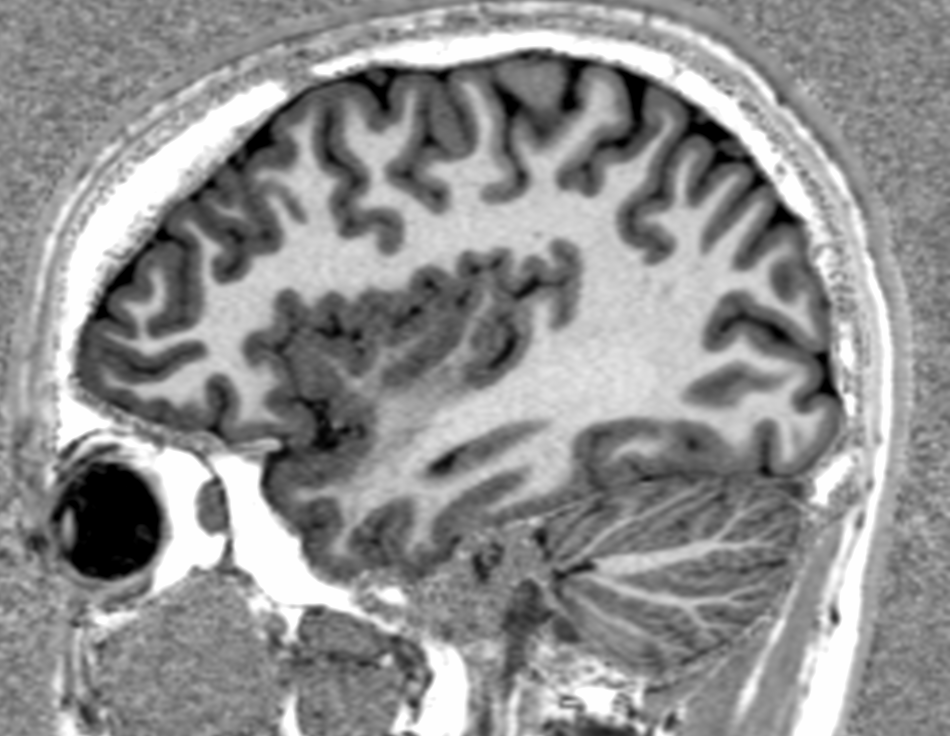
plotting.plot_anat(T2_filename, title="T2", vmax=300)| T1w | T2w |
|---|---|
 |
 |
- Different acquisition techniques will offer better quantification of specific brain tissues