Introduction to Diffusion MRI data

---

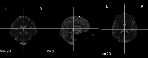
Figure 1

Image 1 of 1: ‘Diffusion along different directions’

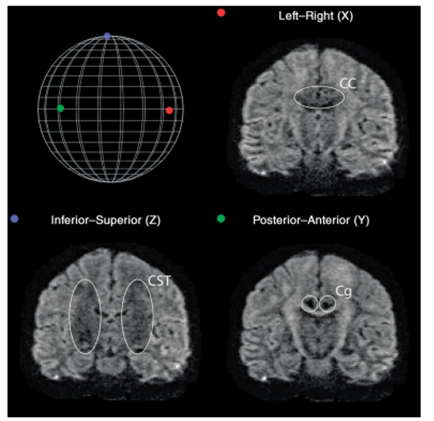
Diffusion along X, Y, and Z directions. The signal in the left/right oriented corpus callosum is lowest when measured along X, while the signal in the inferior/superior oriented corticospinal tract is lowest when measured along Z.

---

Figure 2

Image 1 of 1: ‘DWI slice’

---

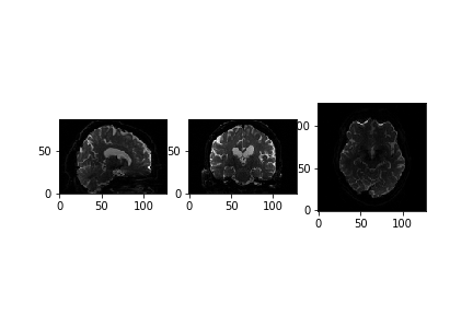
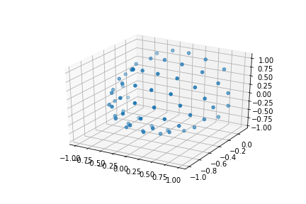
Figure 3

Image 1 of 1: ‘Diffusion gradient sphere’

---

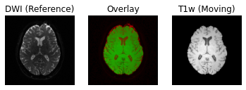
Preprocessing dMRI data

---

Figure 1

Image 1 of 1: ‘Preprocessing steps’

To illustrate what the preprocessing step may look like, here is an example preprocessing workflow from QSIPrep (Cieslak et al, 2020):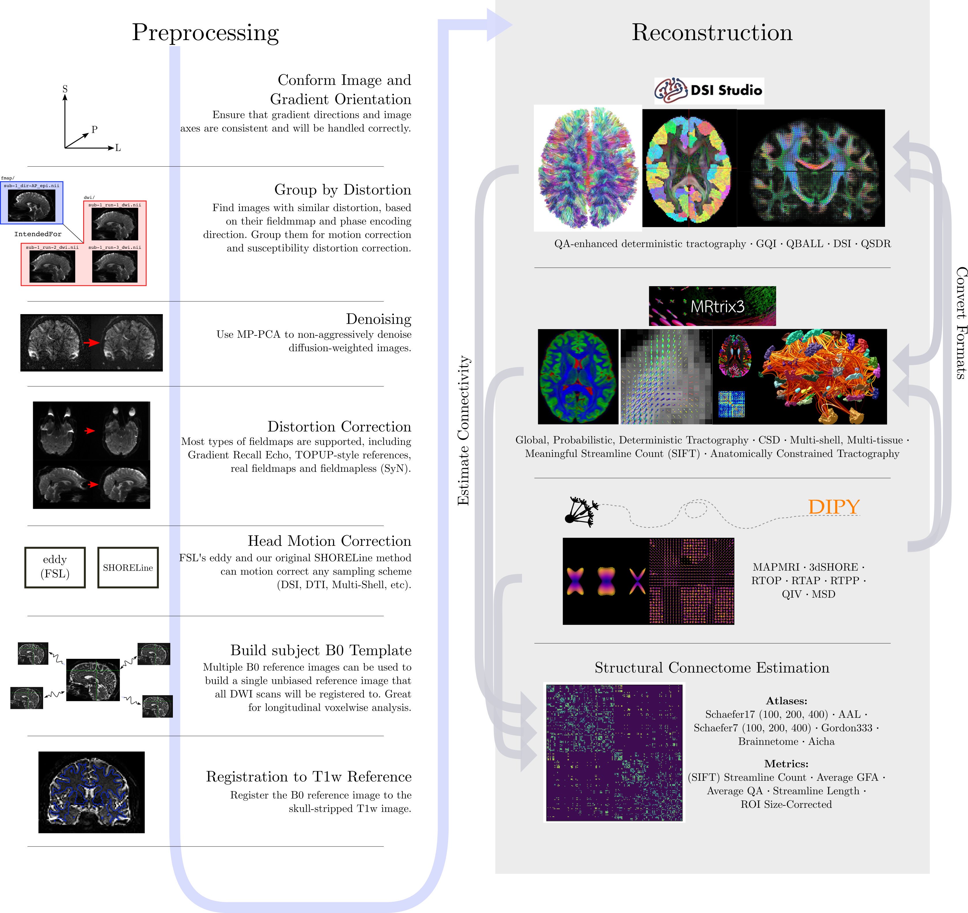

---

Figure 2

Image 1 of 1: ‘b0 brainmask’

---

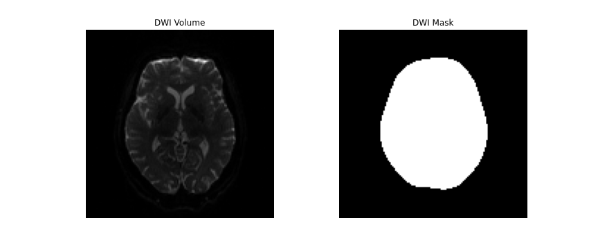
Figure 3

Image 1 of 1: ‘Blip up and blip down pairs’

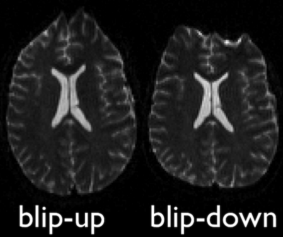
Opposite phase-encodings from two DWI

---

Figure 4

Image 1 of 1: ‘Topup image’

---

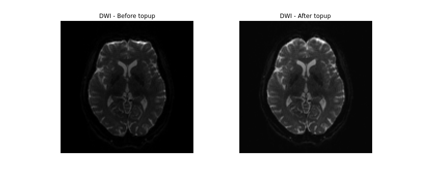
Figure 5

Image 1 of 1: ‘T1w brainmask’

---

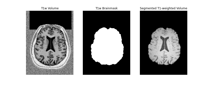
Figure 6

Image 1 of 1: ‘Transformed volumes’

---

Local fiber orientation reconstruction

---

Diffusion Tensor Imaging (DTI)

---

Figure 1

Image 1 of 1: ‘Diffusion signal equation’

---

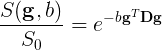
Figure 2

Image 1 of 1: ‘Diffusivity matrix’

---

Figure 3

Image 1 of 1: ‘Diffusion tensor’

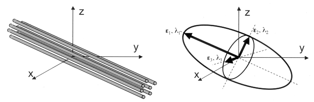Adapted from Jelison et al., 2004

---

Figure 4

Image 1 of 1: ‘FA equation’

---

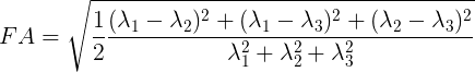
Figure 5

Image 1 of 1: ‘FA plot’

---

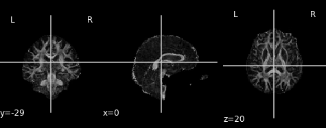
Figure 6

Image 1 of 1: ‘MD equation’

---

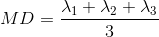
Figure 7

Image 1 of 1: ‘MD plot’

---

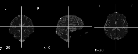
Figure 8

Image 1 of 1: ‘Axial and radial diffusivities’

---

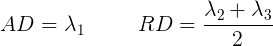
Figure 9

Image 1 of 1: ‘RGB FA map’

---

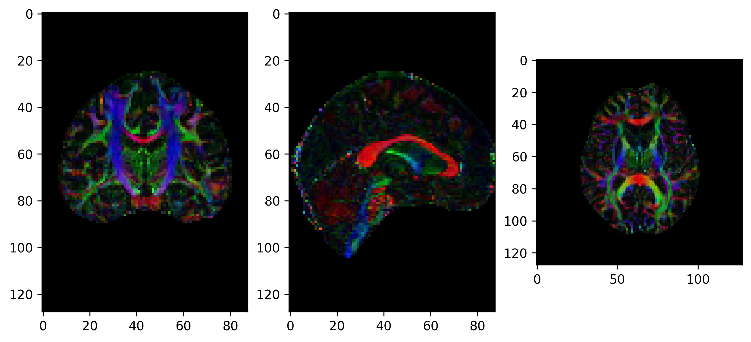
Figure 10

Image 1 of 1: ‘Tensor visualization’

---

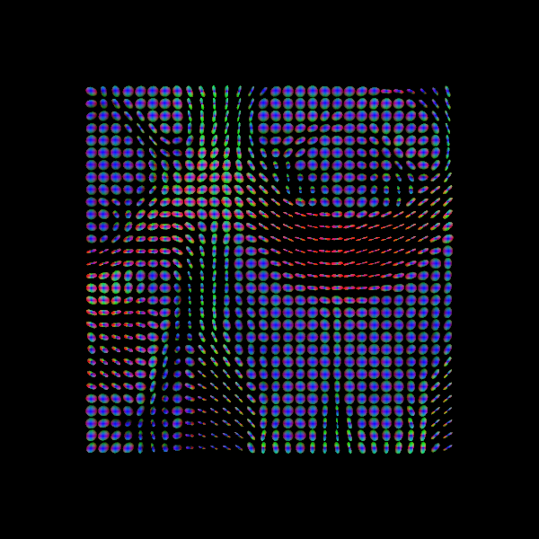
Figure 11

Image 1 of 1: ‘DTI drawbacks’

---

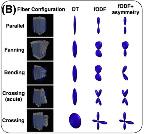
Figure 12

Image 1 of 1: ‘Axial diffusivity map’

Axial diffusivity map.

---

Figure 13

Image 1 of 1: ‘Radial diffusivity map’

Radial diffusivity map.

---

Constrained Spherical Deconvolution (CSD)

---

Figure 1

Image 1 of 1: ‘Spherical deconvolution equation’

The basic equations of an SD method can be summarized as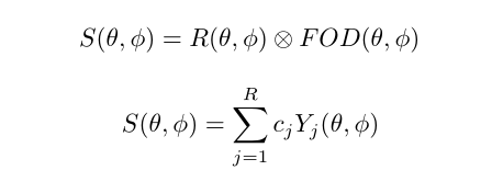
Spherical deconvolution

---

Figure 2

Image 1 of 1: ‘Fiber Response Function (FRF)’

Estimated response function

---

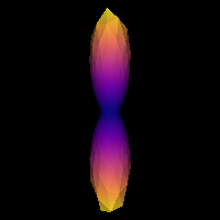
Figure 3

Image 1 of 1: ‘CSD ODFs’

CSD ODFs.

---

Figure 4

Image 1 of 1: ‘CSD peaks’

CSD Peaks.

---

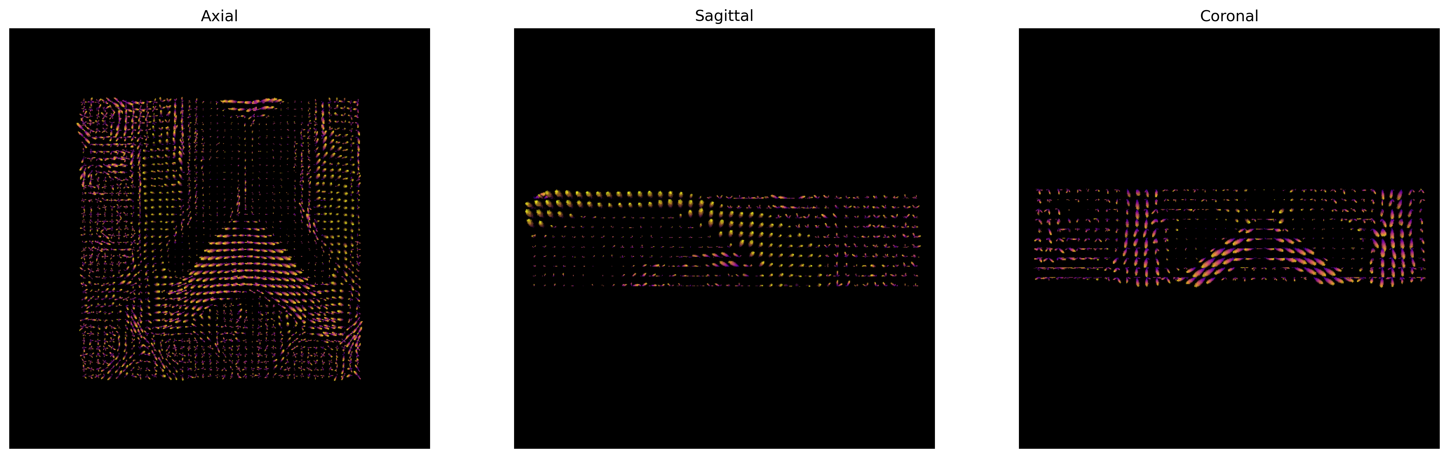
Figure 5

Image 1 of 1: ‘CSD peaks and fODFs’

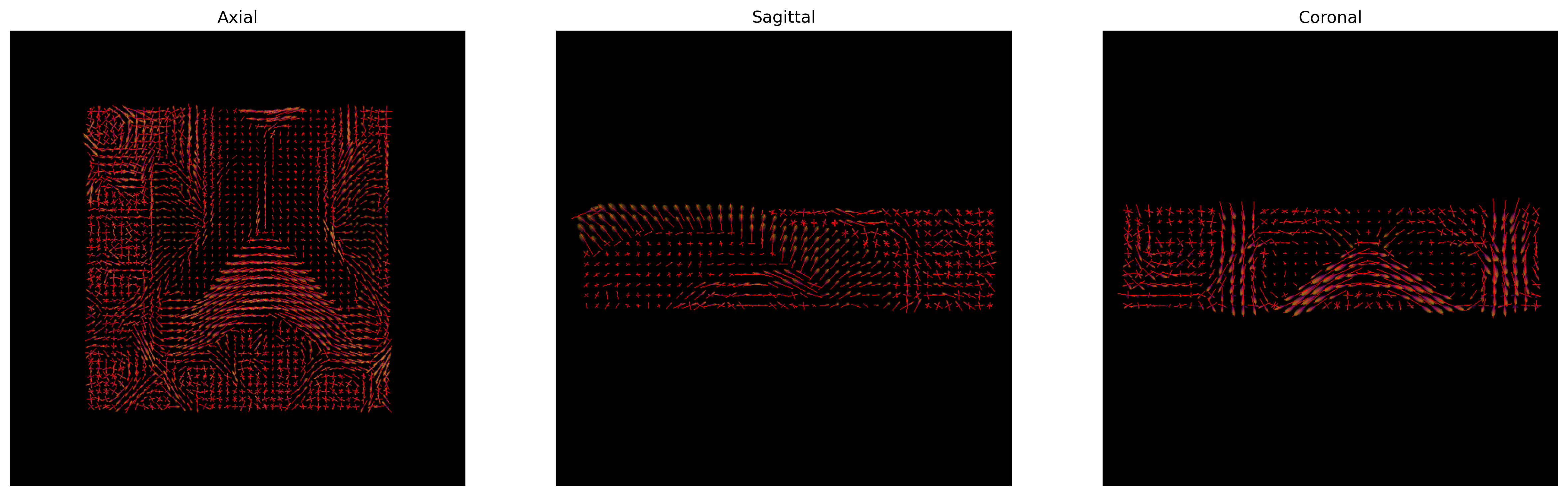
CSD Peaks and ODFs.

---

Figure 6

Image 1 of 1: ‘ODFs of differing crossing angles’

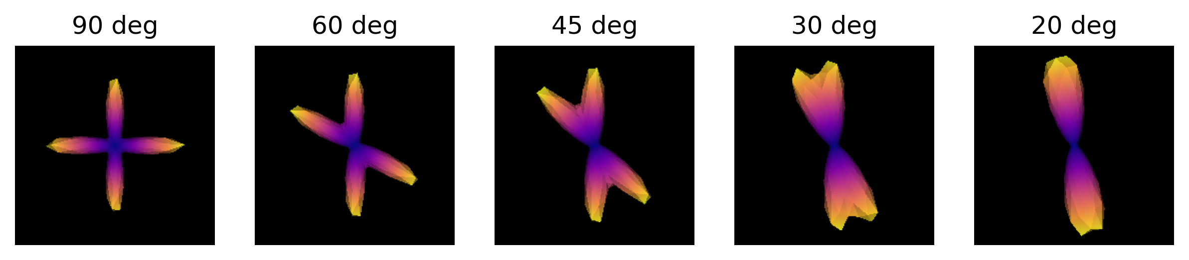
ODFs of different crossing angles.

---

Tractography

---

Local tractography

---

Figure 1

Image 1 of 1: ‘Streamline propagation equation’

Streamline propagation is, in essence, a numerical analysis integration problem. The problem lies in finding a curve that joins a set of discrete local directions. As such, it takes the form of a differential equation problem of the form: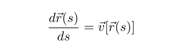
Streamline propagation differential equation

---

Deterministic tractography

---

Figure 1

Image 1 of 1: ‘FA’

---

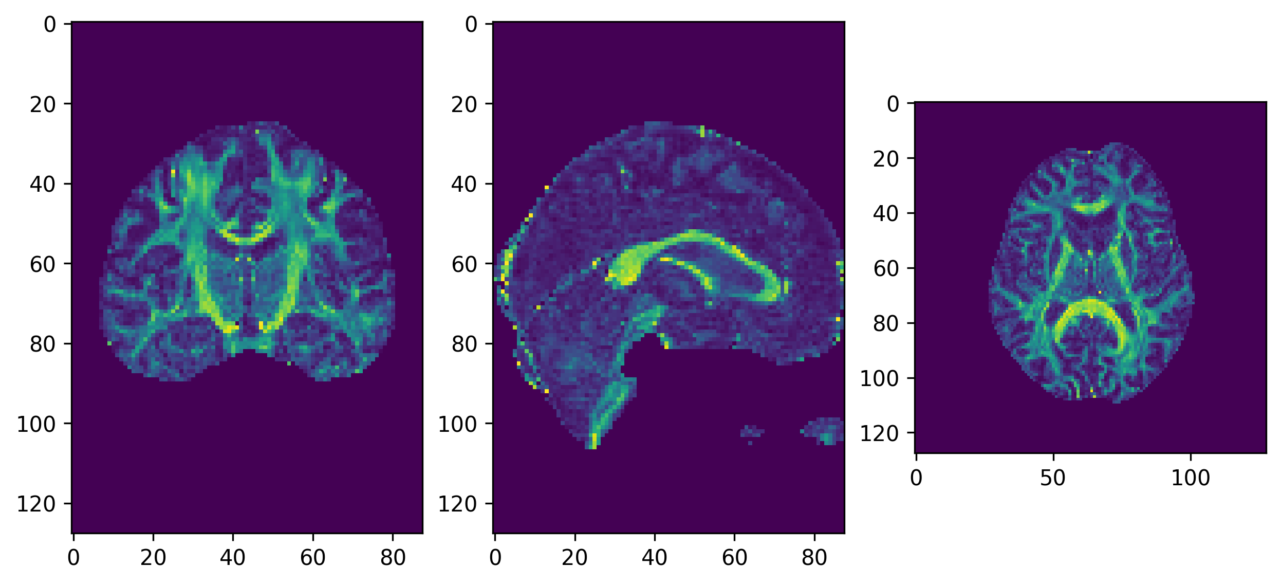
Figure 2

Image 1 of 1: ‘EuDX Determinsitic Tractography’

---

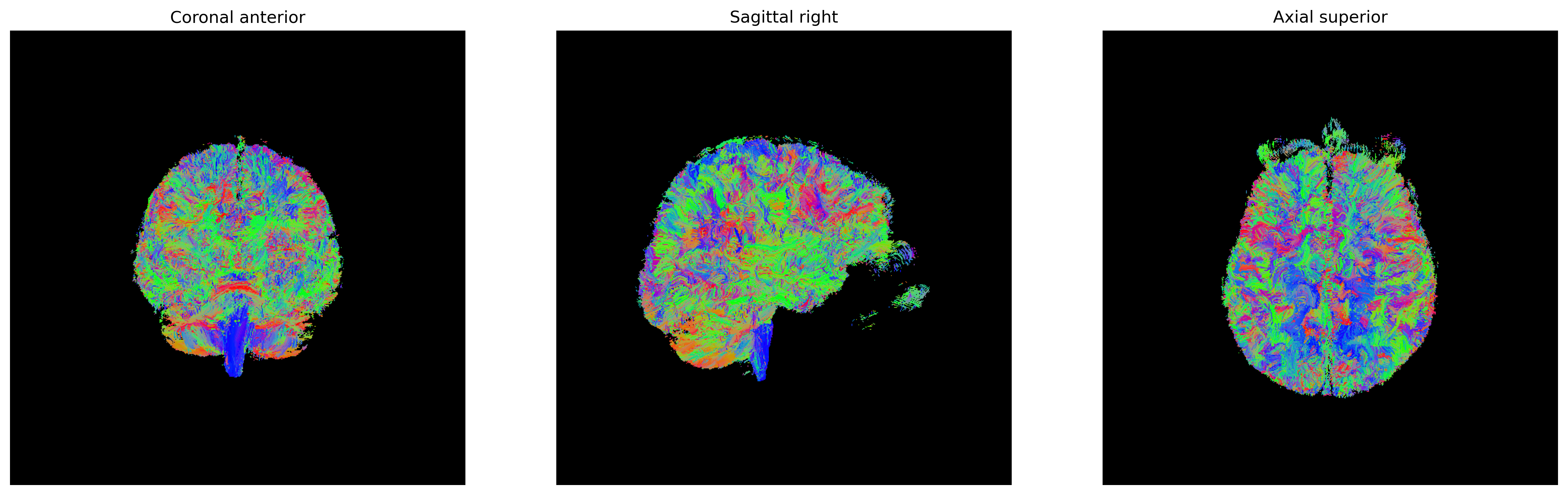
Figure 3

Image 1 of 1: ‘Binary Stopping Criterion Tractography’

---

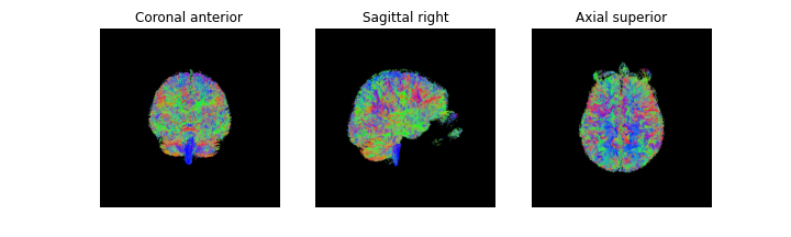
Figure 4

Image 1 of 1: ‘FA Mapped Tractography’

---

Probabilistic tractography

---

Figure 1

Image 1 of 1: ‘GFA’

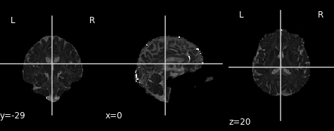
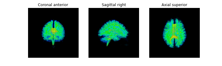
GFA

---

Figure 2

Image 1 of 1: ‘PMF direction getter-derived probabilistic tractogram’

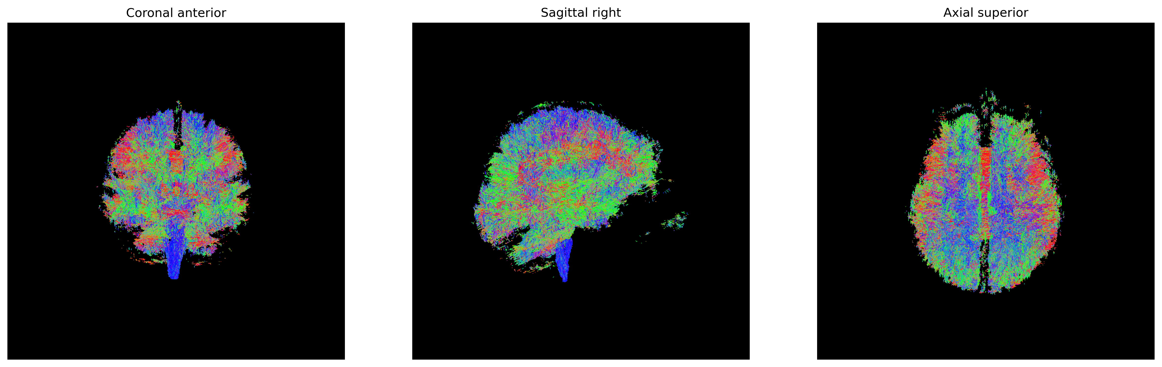
Streamlines representing white matter using probabilistic direction getter from PMF

---

Figure 3

Image 1 of 1: ‘SH direction getter-derived probabilistic tractogram’

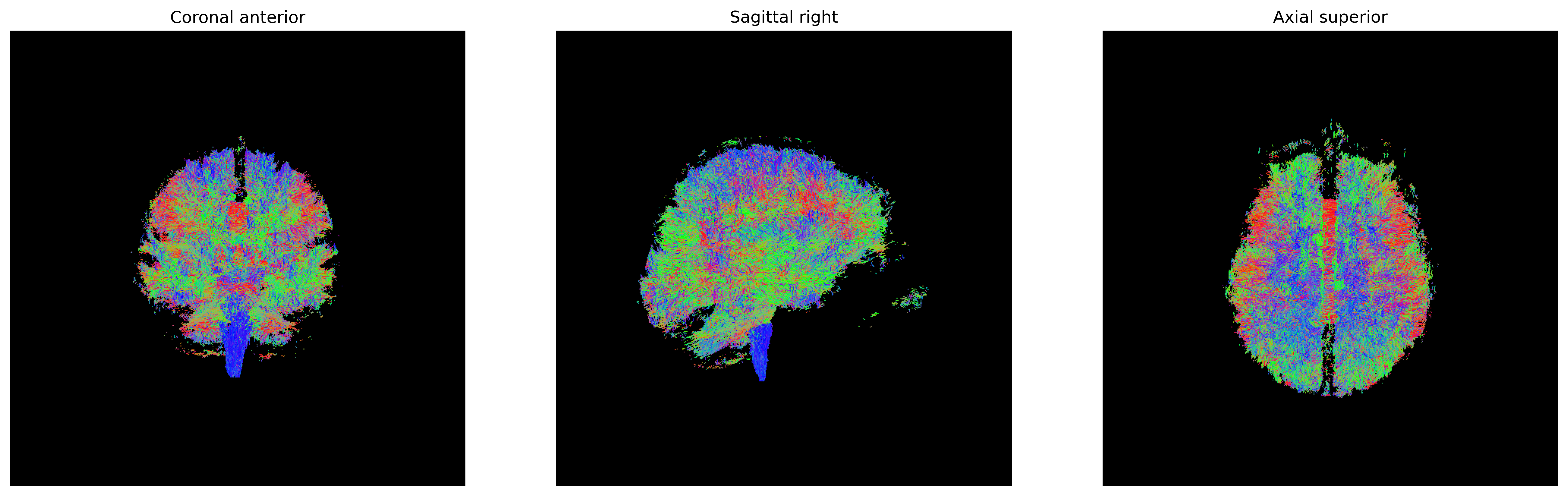
Streamlines representing white matter using probabilistic direction getter from SH

---

Figure 4

Image 1 of 1: ‘CSD model peaks for tracking’

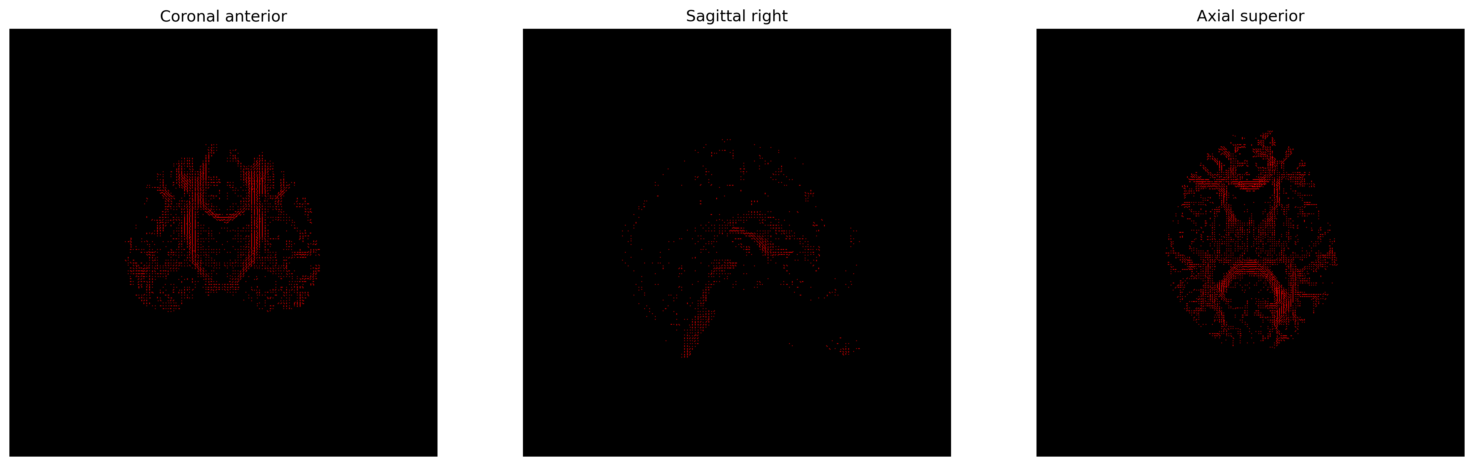
Peaks obtained from the CSD model for tracking purposes

---

Figure 5

Image 1 of 1: ‘PMF SH direction getter-derived probabilistic tractogram’

Streamlines representing white matter using probabilistic direction getter from SH (peaks_from_model)

---