
Stan extensions
Last updated on 2026-08-10 | Edit this page
Overview
Questions
- Which packages take advantage of Stan and how to use them?
Objectives
- Learn to use Stan with additional R packages
In this chapter, we will introduce packages that take advantage of
Stan. The covered packages are loo, which enables
approximate Bayesian cross-validation, bayesplot, which
contains plotting tools, and brms, which allows calling
Stan using common R syntax, without having to write the Stan code.
loo
The loo package allows computing approximate
leave-one-out cross-validation (loo-cv) for models fitted with Stan. The
approximation is based on something called Pareto smoothed importance
sampling (PSIS) [1]. The package can also be used for computing WAIC and
model weights for average predictive distributions.
Example 1
We will demonstrate loo package usage on the model
comparison example studied in Episode 5. We will fit the normal and
Cauchy models on the same synthetic data, then use the tools provided in
loo to compute and compare the approximate loo-cv scores
for these two models.
To be able to utilize the package functions, we need to add a
log-likelihood computation in the Stan code, in the generated quantities
block. The generated quantities block computes the pointwise
log-likelihood, stored in a variable named log_lik.
CmdStanR automatically recognizes this variable, allowing the loo
package to compute approximate leave-one-out cross-validation. Below, we
demonstrate this with the two models we are comparing.
STAN
// Normal model
data {
  int<lower=0> N;
  vector[N] X;
}
parameters {
  real<lower=0> sigma;
  real mu;
}
model {
  X ~ normal(mu, sigma);

  mu ~ normal(0, 1);
  sigma ~ gamma(2, 1);
}

generated quantities {
  vector[N] X_rep;

  for(i in 1:N) {
    X_rep[i] = normal_rng(mu, sigma);
  }

  // Calculating log-likelihood for loo
  vector[N] log_lik;

  for (i in 1:N) {
  log_lik[i] = normal_lpdf(X[i] | mu, sigma);
  }
}
STAN
// Cauchy model
data {
  int<lower=0> N;
  vector[N] X;
}
parameters {
  // Scale
  real<lower=0> sigma;
  // location
  real mu;
}
model {
  // location = mu and scale = sigma
  X ~ cauchy(mu, sigma);

  mu ~ normal(0, 1);
  sigma ~ gamma(2, 1);
}
generated quantities {
  vector[N] X_rep;
  for(i in 1:N) {
    X_rep[i] = cauchy_rng(mu, sigma);
  }

  // Calculating log-likelihood for loo
  vector[N] log_lik;

  for (i in 1:N) {
  log_lik[i] = cauchy_lpdf(X[i] | mu, sigma);
  }
}
Now we can fit the models in the usual way.
R
# Fit normal model
normal_fit <- normal_model_loo$sample(
                       data = list(N = N, X = df5$X),
                       refresh = 0,
                       seed = 2024
                       )
# Fit cauchy model
cauchy_fit <- cauchy_model_loo$sample(
                       data = list(N = N, X = df5$X),
                       refresh = 0,
                       seed = 2024
                       )
We can now compute PSIS-LOO for both of the models with
loo::loo function. After the calling the function,
information about the fit can be viewed by printing the loo
objects.
R
# PSIS-LOO computation for normal model
normal_loo <- normal_fit$loo()
WARNING
Warning: Some Pareto k diagnostic values are too high. See help('pareto-k-diagnostic') for details.R
print(normal_loo)
OUTPUT
Computed from 4000 by 88 log-likelihood matrix.

         Estimate   SE
elpd_loo   -289.1 41.8
p_loo        18.3 17.3
looic       578.3 83.7
------
MCSE of elpd_loo is NA.
MCSE and ESS estimates assume MCMC draws (r_eff in [0.8, 0.9]).

Pareto k diagnostic values:
                         Count Pct.    Min. ESS
(-Inf, 0.7]   (good)     87    98.9%   2295
   (0.7, 1]   (bad)       0     0.0%   <NA>
   (1, Inf)   (very bad)  1     1.1%   <NA>
See help('pareto-k-diagnostic') for details.
R
# PSIS-LOO computation for cauchy model
cauchy_loo <- cauchy_fit$loo()
print(cauchy_loo)
OUTPUT
Computed from 4000 by 88 log-likelihood matrix.

         Estimate   SE
elpd_loo   -206.9 14.7
p_loo         1.9  0.0
looic       413.7 29.4
------
MCSE of elpd_loo is 0.0.
MCSE and ESS estimates assume MCMC draws (r_eff in [0.7, 0.9]).

All Pareto k estimates are good (k < 0.7).
See help('pareto-k-diagnostic') for details.
Running print returns \(\widehat{\text{elpd}}_{\text{loo}}\)
(expected log pointwise predictive density), \(\hat{p}_{loo}\) (estimated number of
parameters) and \(\text{looic}\) (LOO
information criterion) values and their standard errors. It also returns
a table with the Pareto \(k\)
diagnostic values, which are used to asses the reliability of the
estimates. Values below 1 are required for reliable PSIS estimates.
Model comparison can be done by using the
loo::loo_compare function on the loo objects.
The comparison is based on the models’ elpd values.
R
# Comparing models based on loo
loo::loo_compare(normal_loo, cauchy_loo)
OUTPUT
  model elpd_diff se_diff p_worse diag_diff      diag_elpd
 model2       0.0     0.0      NA
 model1     -82.3    36.4    0.99   N < 100 1 k_psis > 0.7
OUTPUT
Diagnostic flags present.
See ?`loo-glossary` (sections `diag_diff` and `diag_elpd`)
or https://mc-stan.org/loo/reference/loo-glossary.html.
The comparison shows that the elpd difference is larger than the standard error, indicating that the cauchy model is expected to have better predictive performance than the normal model. This is in line with what we saw in chapter 5: the Cauchy distribution is a superior model for the data.
Challenge
loo can also be used to compute WAIC for Bayesian
models. Calculate WAIC for the two models and then compare them.
First we need to extract the log-likelihood values from the fitted
model object using draws().
R
# Extracting loglik
normal_loglik <- normal_fit$draws("log_lik", format = "matrix")
cauchy_loglik <- cauchy_fit$draws("log_lik", format = "matrix")

# Computing WAIC for the models
normal_waic <- loo::waic(normal_loglik)
WARNING
Warning:
1 (1.1%) p_waic estimates greater than 0.4. We recommend trying loo instead.
R
print(normal_waic)
OUTPUT
Computed from 4000 by 88 log-likelihood matrix.

          Estimate   SE
elpd_waic   -292.3 45.0
p_waic        21.4 20.5
waic         584.6 89.9

1 (1.1%) p_waic estimates greater than 0.4. We recommend trying loo instead.
R
cauchy_waic <- loo::waic(cauchy_loglik)
print(cauchy_waic)
OUTPUT
Computed from 4000 by 88 log-likelihood matrix.

          Estimate   SE
elpd_waic   -206.9 14.7
p_waic         1.9  0.0
waic         413.7 29.4
Computing WAIC for the model return values for \(\widehat{\text{eldp}}_{\text{WAIC}}\), \(\hat{p}_{\text{WAIC}}\) and \(\widehat{\text{WAIC}}\). Models can be compared based on WAIC using the same function as with PSIS-LOO.
R
# Comparing models based on WAIC
loo::loo_compare(normal_waic, cauchy_waic)
OUTPUT
  model elpd_diff se_diff p_worse diag_diff diag_elpd
 model2       0.0     0.0      NA
 model1     -85.4    39.5    0.98   N < 100
OUTPUT
Diagnostic flags present.
See ?`loo-glossary` (sections `diag_diff` and `diag_elpd`)
or https://mc-stan.org/loo/reference/loo-glossary.html.
bayesplot
Next, we will look at the the bayesplot R package. The
package provides a library of plotting functions for fitted Stan models.
The created plots are ggplot objects, meaning that the
plots can be customized with the functions from ggplot2
package. The package enables plotting posterior draws, visual MCMC
diagnostics and graphical posterior and prior predictive checking. The
functions of the package also work with model fit with the popular
packages brms and rstanarm.
Example 1 continued
We will demonstrate using bayesplot with the Cauchy
model used in the first example. First, we need to extract the posterior
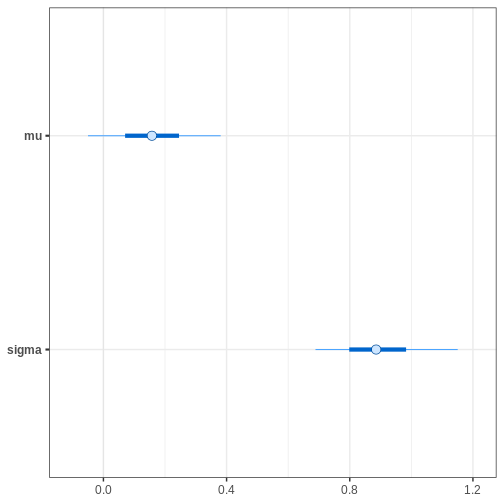
draws. Then, we will plot uncertainty intervals for \(\mu\) and \(\sigma\).
R
# Extracting draws
cauchy_draws <- cauchy_fit$draws()

# Plotting uncertainty intervals
bayesplot::mcmc_intervals(cauchy_draws, pars = c("mu", "sigma"))
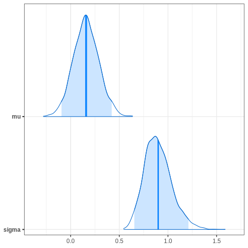
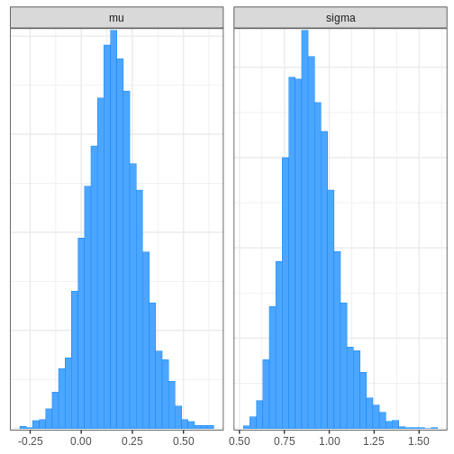
Alternatively, we can plot the (marginal) posterior sample histograms or densities with credible intervals as shaded areas as follows:
R
# Plotting estimated density curves
bayesplot::mcmc_areas(cauchy_draws, pars = c("mu", "sigma"),
                      prob = 0.95,
                      point_est = "mean")
R
# Plotting histogram
bayesplot::mcmc_hist(cauchy_draws, pars = c("mu", "sigma"))
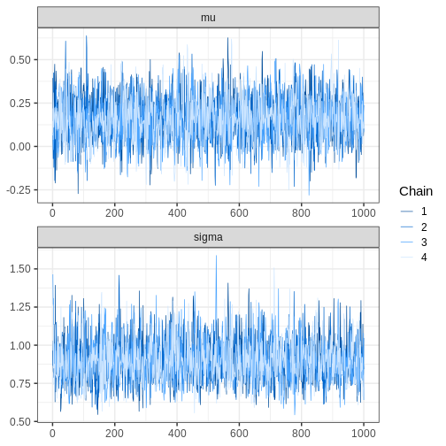
bayesplot also provides functions for assessing MCMC
convergence and visualizing fit diagnostics. For example, we can
generate trace plots for the chains:
R
# Plotting trace plot
bayesplot::mcmc_trace(cauchy_draws, pars = c("mu", "sigma"),
                      facet_args = list(ncol = 1))
Challenge
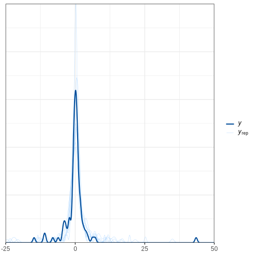
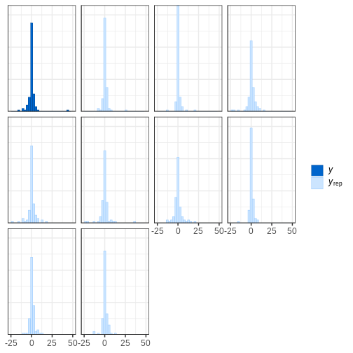
Perform a graphical posterior predictive checks with
bayesplot. Using the Cauchy model fit generated above, plot
the density of \(X_{rep}\) samples
overlaid with the density of \(X\).
Alternatively, you can plot the corresponding histograms.
R
# Extracting replicates and getting a subset
set.seed(2024)
X_rep <- cauchy_fit$draws("X_rep", format = "matrix")

N_rep <- 9

selected_samples <- sample(1:nrow(X_rep), size = N_rep, replace = FALSE)
X_rep_sub <- X_rep[selected_samples, ]
R
# Plot density
# Limit x range for better illustration
bayesplot::ppc_dens_overlay(y = df5$X, yrep = X_rep_sub) + xlim(-25, 50)
R
# Plot histograms
bayesplot::ppc_hist(y = df5$X, yrep = X_rep_sub) + xlim(-25,50)
brms R package
We will now introduce the brms R package. The package
allows fitting probabilistic generalized (non-)linear models with Stan.
A large range of distributions and link functions are supported, in
addition to multilevel structure. Moreover, several built-in functions
are available for priors.
Models are specified using familiar R formula syntax. Throughout this
lesson, brms uses CmdStanR as the backend to
compile and fit the corresponding Stan models.
The package also provides tools for evaluating the fit and MCMC
convergence. These tools, in turn, use functions from the
loo and bayesplot packages, that is, many of
the same tools we covered earlier in this Episode.
Next, we will demonstrate usage of the package with two different examples.
Example 2: Survival modeling
In this example, we will demonstrate fitting a Cox proportional
hazard model with brms. However, first, we will briefly
describe and model and idea in survival modeling.
The Cox model is a standard approach used in survival modeling, in which the outcome of interest is the time to some event. A common application is medical studies where patients are followed in time until an event (e.g. death) or until censoring. A subject is censored if the event doesn’t occur during the follow-up.
An important ingredient in survival modeling is the hazard function, representing the instantaneous risk for an event at time \(t\), defined as \(\lambda(t)=\text{lim}_{h \to 0+} \frac{1}{h}P(t \le T<t+h|T\ge t)\). In the Cox model, the hazard function is of the form \(\lambda(t_i,Z_i,\theta)=\lambda_0(t_i)\text{exp}(\beta^\prime Z_i)\).
The baseline hazard function \(\lambda_0(t_i)\) represents the hazard when the covariates are set to their baselines, and is the same for each subject \(i\). Commonly, the functional form the baseline hazard is not specified. The second part of the hazard function contains subject-specific covariates, \(\text{exp}(\beta^\prime Z_i)\).
The exponentials of the effects \(\beta\) are called hazard ratios, which measure the hazard in one group against the hazard in another group.
When fitting the Cox model, brms uses M-splines for the
baseline hazard. Splines are functions built from piecewise-defined
polynomials. In other words, the baseline hazard is a combination of
several different polynomial functions. M-splines are non-negative
spline functions, which is important for reasons we omit. However,
hopefully, the reader can appreciate the simplicity of the upcoming
brms function call.
Before fitting the model, we will take a look at the
lung dataset from the survival R package,
which we will be analyzing below. The dataset consists of survival times
of patients with advanced lung cancer including some clinical
covariates.
R
# Get data
lung <- survival::lung

# Take a peek
head(lung)
OUTPUT
  inst time status age sex ph.ecog ph.karno pat.karno meal.cal wt.loss
1    3  306      2  74   1       1       90       100     1175      NA
2    3  455      2  68   1       0       90        90     1225      15
3    3 1010      1  56   1       0       90        90       NA      15
4    5  210      2  57   1       1       90        60     1150      11
5    1  883      2  60   1       0      100        90       NA       0
6   12 1022      1  74   1       1       50        80      513       0
The variable status denotes if an event (death) was
observed or if the subject was censored. We will use three covariates:
age, sex and ph.karno. The
variable ph.karno describes how well a patient can perform
daily activities rated by a physician. We will split the variable into
two categories “high” and “low.”
Cox model can be fit with brms::brm() function by
specifying family = brmsfamily("cox"). Censored data points
are indicated with the cens(1 - status) argument. We will
use a standard \(\text{Normal}(0, 10)\)
prior for the population-level effects, with the argument
prior(normal(0,10), class = b). The option
class = b sets the prior for all population-level
effects.
R
# Let's change status coding from 2/1 to 1/0
lung$status <- lung$status - 1

# Remove observations with NA ph.karno
lung <- lung[!is.na(lung$ph.karno),]

# Creating new variable for ph.karno status
lung$ph.karno_status <- cut(lung$ph.karno,
                            breaks = c(0, 70, 100),
                            labels = c("low", "high"))

# Fitting the model
fit_cox <- brms::brm(
  time | cens(1 - status) ~ sex + age + ph.karno_status,
  data = lung,
  family = brmsfamily("cox"),
  backend = "cmdstanr",
  seed = 2024,
  silent = 2,
  refresh = 0,
  cores = 4,
  prior = prior(normal(0, 10), class = b)
)
OUTPUT
Loading required namespace: rstanR
# Summary of the fit
summary(fit_cox)
OUTPUT
 Family: cox
  Links: mu = log
Formula: time | cens(1 - status) ~ sex + age + ph.karno_status
   Data: lung (Number of observations: 227)
  Draws: 4 chains, each with iter = 2000; warmup = 1000; thin = 1;
         total post-warmup draws = 4000

Regression Coefficients:
                    Estimate Est.Error l-95% CI u-95% CI Rhat Bulk_ESS Tail_ESS
Intercept               1.27      0.68    -0.06     2.57 1.00     3410     2831
sex                    -0.51      0.17    -0.83    -0.19 1.00     3155     2579
age                     0.01      0.01    -0.01     0.03 1.00     3691     2925
ph.karno_statushigh    -0.36      0.18    -0.70     0.00 1.00     2931     2453

Draws were sampled using sample(hmc). For each parameter, Bulk_ESS
and Tail_ESS are effective sample size measures, and Rhat is the potential
scale reduction factor on split chains (at convergence, Rhat = 1).
The summary output of the brms fit prints coefficient
estimates, and also returns Rhat, Bulk_ESS and Tail_ESS values, which
can be used to assess the convergence of the model.
It is important to notice that the coefficients are the log hazard
ratios, which means we still need to exponentiate them. The
bayesplot::mcmc_intervals() function allows transforming
the parameters before plotting with transform = "exp"
argument.
R
# Get hazard values
sum_cox <- summary(fit_cox)
exp(sum_cox$fixed[,1:4])
OUTPUT
                     Estimate Est.Error  l-95% CI   u-95% CI
Intercept           3.5449935  1.966953 0.9441448 13.0026137
sex                 0.6028369  1.182707 0.4348941  0.8310266
age                 1.0131731  1.009298 0.9947433  1.0315701
ph.karno_statushigh 0.6960354  1.194420 0.4949508  1.0021477
R
# Credible intervals
bayesplot::mcmc_intervals(fit_cox,
                          pars = c("b_sex", "b_age", "b_ph.karno_statushigh"),
                          transform = "exp")
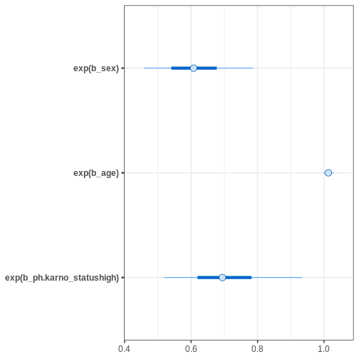
Based on the estimates, it seems that age has only a minor effect on
the hazard. Female sex and being “high” in ph.karno imply
smaller hazards, meaning that these factors are protective.
After fitting the model, we can print information about the priors
used with the function brms::get_prior.
R
# Get priors for the cox model
brms::get_prior(fit_cox)
OUTPUT
                  prior     class                coef group resp dpar nlpar lb
                 (flat)         b
                 (flat)         b                 age
                 (flat)         b ph.karno_statushigh
                 (flat)         b                 sex
 student_t(3, 5.6, 2.5) Intercept
           dirichlet(1)     sbhaz
 ub tag       source
             default
        (vectorized)
        (vectorized)
        (vectorized)
             default
             default
The population-level effects have the normal prior we specified. In
brms, the default prior for the intercept is Student’s
t-distribution with three degrees of freedom. The Stan program generated
by brms can be inspected using
brms::stancode(). When backend = "cmdstanr" is
used, this Stan program is compiled and sampled with CmdStan.
R
# Print the Stan code
brms::stancode(fit_cox)
OUTPUT
// generated with brms 2.23.0
functions {
  /* distribution functions of the Cox proportional hazards model
   * parameterize hazard(t) = baseline(t) * mu
   * so that higher values of 'mu' imply lower survival times
   * Args:
   *   y: the response value; currently ignored as the relevant
   *     information is passed via 'bhaz' and 'cbhaz'
   *   mu: positive location parameter
   *   bhaz: baseline hazard
   *   cbhaz: cumulative baseline hazard
   */
  real cox_lhaz(real y, real mu, real bhaz, real cbhaz) {
    return log(bhaz) + log(mu);
  }
  vector cox_lhaz(vector y, vector mu, vector bhaz, vector cbhaz) {
    return log(bhaz) + log(mu);
  }

  // equivalent to the log survival function
  real cox_lccdf(real y, real mu, real bhaz, real cbhaz) {
    return - cbhaz * mu;
  }
  real cox_lccdf(vector y, vector mu, vector bhaz, vector cbhaz) {
    return - dot_product(cbhaz, mu);
  }

  real cox_lcdf(real y, real mu, real bhaz, real cbhaz) {
    return log1m_exp(cox_lccdf(y | mu, bhaz, cbhaz));
  }
  real cox_lcdf(vector y, vector mu, vector bhaz, vector cbhaz) {
    return sum(log1m_exp(- cbhaz .* mu));
  }

  real cox_lpdf(real y, real mu, real bhaz, real cbhaz) {
    return cox_lhaz(y, mu, bhaz, cbhaz) + cox_lccdf(y | mu, bhaz, cbhaz);
  }
  real cox_lpdf(vector y, vector mu, vector bhaz, vector cbhaz) {
    return sum(cox_lhaz(y, mu, bhaz, cbhaz)) + cox_lccdf(y | mu, bhaz, cbhaz);
  }

  // Distribution functions of the Cox model in log parameterization
  real cox_log_lhaz(real y, real log_mu, real bhaz, real cbhaz) {
    return log(bhaz) + log_mu;
  }
  vector cox_log_lhaz(vector y, vector log_mu, vector bhaz, vector cbhaz) {
    return log(bhaz) + log_mu;
  }

  real cox_log_lccdf(real y, real log_mu, real bhaz, real cbhaz) {
    return - cbhaz * exp(log_mu);
  }
  real cox_log_lccdf(vector y, vector log_mu, vector bhaz, vector cbhaz) {
    return - dot_product(cbhaz, exp(log_mu));
  }

  real cox_log_lcdf(real y, real log_mu, real bhaz, real cbhaz) {
    return log1m_exp(cox_log_lccdf(y | log_mu, bhaz, cbhaz));
  }
  real cox_log_lcdf(vector y, vector log_mu, vector bhaz, vector cbhaz) {
    return sum(log1m_exp(- cbhaz .* exp(log_mu)));
  }

  real cox_log_lpdf(real y, real log_mu, real bhaz, real cbhaz) {
    return cox_log_lhaz(y, log_mu, bhaz, cbhaz) +
           cox_log_lccdf(y | log_mu, bhaz, cbhaz);
  }
  real cox_log_lpdf(vector y, vector log_mu, vector bhaz, vector cbhaz) {
    return sum(cox_log_lhaz(y, log_mu, bhaz, cbhaz)) +
           cox_log_lccdf(y | log_mu, bhaz, cbhaz);
  }
}
data {
  int<lower=1> N;  // total number of observations
  vector[N] Y;  // response variable
  // censoring indicator: 0 = event, 1 = right, -1 = left, 2 = interval censored
  array[N] int<lower=-1,upper=2> cens;
  int<lower=1> K;  // number of population-level effects
  matrix[N, K] X;  // population-level design matrix
  int<lower=1> Kc;  // number of population-level effects after centering
  // data for flexible baseline functions
  int Kbhaz;  // number of basis functions
  // design matrix of the baseline function
  matrix[N, Kbhaz] Zbhaz;
  // design matrix of the cumulative baseline function
  matrix[N, Kbhaz] Zcbhaz;
  // a-priori concentration vector of baseline coefficients
  vector<lower=0>[Kbhaz] con_sbhaz;
  int prior_only;  // should the likelihood be ignored?
}
transformed data {
  // indices of censored data
  int Nevent = 0;
  int Nrcens = 0;
  int Nlcens = 0;
  array[N] int Jevent;
  array[N] int Jrcens;
  array[N] int Jlcens;
  matrix[N, Kc] Xc;  // centered version of X without an intercept
  vector[Kc] means_X;  // column means of X before centering
  // collect indices of censored data
  for (n in 1:N) {
    if (cens[n] == 0) {
      Nevent += 1;
      Jevent[Nevent] = n;
    } else if (cens[n] == 1) {
      Nrcens += 1;
      Jrcens[Nrcens] = n;
    } else if (cens[n] == -1) {
      Nlcens += 1;
      Jlcens[Nlcens] = n;
    }
  }
  for (i in 2:K) {
    means_X[i - 1] = mean(X[, i]);
    Xc[, i - 1] = X[, i] - means_X[i - 1];
  }
}
parameters {
  vector[Kc] b;  // regression coefficients
  real Intercept;  // temporary intercept for centered predictors
  // baseline hazard coefficients
  simplex[Kbhaz] sbhaz;
}
transformed parameters {
  // prior contributions to the log posterior
  real lprior = 0;
  lprior += normal_lpdf(b | 0, 10);
  lprior += student_t_lpdf(Intercept | 3, 5.6, 2.5);
  lprior += dirichlet_lpdf(sbhaz | con_sbhaz);
}
model {
  // likelihood including constants
  if (!prior_only) {
    // compute values of baseline function
    vector[N] bhaz = Zbhaz * sbhaz;
    // compute values of cumulative baseline function
    vector[N] cbhaz = Zcbhaz * sbhaz;
    // initialize linear predictor term
    vector[N] mu = rep_vector(0.0, N);
    mu += Intercept + Xc * b;
    // vectorized log-likelihood contributions of censored data
    target += cox_log_lpdf(Y[Jevent[1:Nevent]] | mu[Jevent[1:Nevent]], bhaz[Jevent[1:Nevent]], cbhaz[Jevent[1:Nevent]]);
    target += cox_log_lccdf(Y[Jrcens[1:Nrcens]] | mu[Jrcens[1:Nrcens]], bhaz[Jrcens[1:Nrcens]], cbhaz[Jrcens[1:Nrcens]]);
    target += cox_log_lcdf(Y[Jlcens[1:Nlcens]] | mu[Jlcens[1:Nlcens]], bhaz[Jlcens[1:Nlcens]], cbhaz[Jlcens[1:Nlcens]]);
  }
  // priors including constants
  target += lprior;
}
generated quantities {
  // actual population-level intercept
  real b_Intercept = Intercept - dot_product(means_X, b);
}
Example 3: Hierarchical binomial model
We will now demonstrate one of the key focuses of brms,
fitting hierarchical models. The syntax for specifying hierarchical
models is similar as in the lme4 package, which is used to
fit frequentist multilevel models in R.
For this example, we will be using is the VerbAgg data
from lme4 package. The data consist of item responses to a
questionnaire on verbal aggression.
R
# Get data
VerbAgg <- lme4::VerbAgg

head(VerbAgg)
OUTPUT
  Anger Gender        item    resp id btype  situ mode r2
1    20      M S1WantCurse      no  1 curse other want  N
2    11      M S1WantCurse      no  2 curse other want  N
3    17      F S1WantCurse perhaps  3 curse other want  Y
4    21      F S1WantCurse perhaps  4 curse other want  Y
5    17      F S1WantCurse perhaps  5 curse other want  Y
6    21      F S1WantCurse     yes  6 curse other want  Y
We will estimate population-level effects for Anger, Gender, btype
and situ, and include a group-level intercept for id. The variable of
interest is the binary r2, which contains the response to an question in
the questionnaire. We will use \(\text{Normal}(0, 10)\) as the prior for all
the population-level effects. For the standard deviation of group-level
effect we will set a (half-)\(\text{Cauchy}(0,
5)\) prior. By default, brms uses half-Student’s
t-distribution with three degrees of freedom for standard deviation
parameters. The group-level intercept for variable id is specified with
the argument (1|id). Let’s now fit the model.
R
# Change coding for r2
VerbAgg <- VerbAgg %>%
  mutate(r2 = ifelse(r2 == "N", 0, 1))
# Fit model
fit_hier <- brms::brm(
  r2 ~ Anger + Gender + btype + situ + (1 | id),
  family = bernoulli,
  data = VerbAgg,
  backend = "cmdstanr",
  seed = 2024,
  cores = 4,
  silent = 2,
  refresh = 0,
  prior = prior(normal(0, 10), class = b) +
    prior(cauchy(0, 5), class = sd)
)
# Summary
summary(fit_hier)
OUTPUT
 Family: bernoulli
  Links: mu = logit
Formula: r2 ~ Anger + Gender + btype + situ + (1 | id)
   Data: VerbAgg (Number of observations: 7584)
  Draws: 4 chains, each with iter = 2000; warmup = 1000; thin = 1;
         total post-warmup draws = 4000

Multilevel Hyperparameters:
~id (Number of levels: 316)
              Estimate Est.Error l-95% CI u-95% CI Rhat Bulk_ESS Tail_ESS
sd(Intercept)     1.30      0.07     1.17     1.44 1.00      987     1615

Regression Coefficients:
           Estimate Est.Error l-95% CI u-95% CI Rhat Bulk_ESS Tail_ESS
Intercept      0.20      0.33    -0.45     0.85 1.00      819     1517
Anger          0.06      0.02     0.02     0.09 1.00      797     1485
GenderM        0.31      0.18    -0.05     0.69 1.00      670     1357
btypescold    -1.03      0.07    -1.17    -0.90 1.00     5190     3467
btypeshout    -2.00      0.07    -2.14    -1.85 1.00     4539     3071
situself      -1.01      0.06    -1.12    -0.89 1.00     6186     2961

Draws were sampled using sample(hmc). For each parameter, Bulk_ESS
and Tail_ESS are effective sample size measures, and Rhat is the potential
scale reduction factor on split chains (at convergence, Rhat = 1).
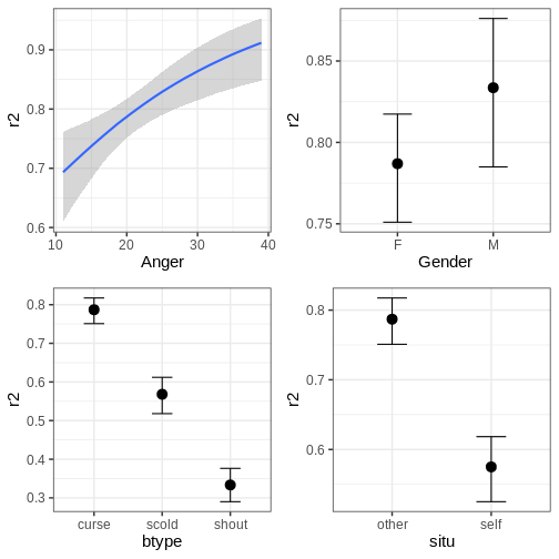
The conditional effects of the predictors can easily be plotted with
the function brms::conditional_effects.
R
# Conditional effects
plots <- suppressMessages(
  plot(brms::conditional_effects(fit_hier), plot = FALSE))
suppressMessages(
cowplot::plot_grid(plots[[1]], plots[[2]], plots[[3]], plots[[4]]))
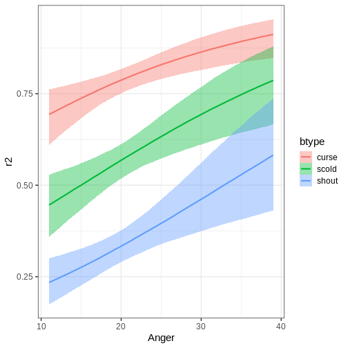
The function can also plot variable interactions. Let’s plot the conditional effect for interaction between Anger and btype.
R
# Plot conditional effect for interaction of Anger and btype
plot(conditional_effects(fit_hier, effects = "Anger:btype"))
Let us now do a slight alteration in model and add another
group-level intercept for the item variable. The priors are same as in
the first model. The update function can be used to modify
the formula without writing it anew in its entirety.
R
# Update model
fit_hier2 <- update(fit_hier, formula. = ~ . + (1|item), newdata = VerbAgg, seed = 2024,
                    cores = 4, silent = 2, refresh = 0, backend = "cmdstanr")
# Summary
summary(fit_hier2)
OUTPUT
 Family: bernoulli
  Links: mu = logit
Formula: r2 ~ Anger + Gender + btype + situ + (1 | id) + (1 | item)
   Data: VerbAgg (Number of observations: 7584)
  Draws: 4 chains, each with iter = 2000; warmup = 1000; thin = 1;
         total post-warmup draws = 4000

Multilevel Hyperparameters:
~id (Number of levels: 316)
              Estimate Est.Error l-95% CI u-95% CI Rhat Bulk_ESS Tail_ESS
sd(Intercept)     1.37      0.07     1.24     1.51 1.00     1307     1834

~item (Number of levels: 24)
              Estimate Est.Error l-95% CI u-95% CI Rhat Bulk_ESS Tail_ESS
sd(Intercept)     0.59      0.11     0.42     0.83 1.00     1327     2222

Regression Coefficients:
           Estimate Est.Error l-95% CI u-95% CI Rhat Bulk_ESS Tail_ESS
Intercept      0.20      0.44    -0.68     1.04 1.01      964     1363
Anger          0.06      0.02     0.02     0.09 1.01      935     1398
GenderM        0.32      0.20    -0.06     0.72 1.00      858     1487
btypescold    -1.06      0.30    -1.65    -0.45 1.00     1235     1617
btypeshout    -2.11      0.31    -2.72    -1.50 1.00     1206     1931
situself      -1.06      0.25    -1.56    -0.59 1.00     1313     1998

Draws were sampled using sample(hmc). For each parameter, Bulk_ESS
and Tail_ESS are effective sample size measures, and Rhat is the potential
scale reduction factor on split chains (at convergence, Rhat = 1).
Another useful aspect of update is that it allows
resampling from the model without having to recompile the model, for
example, using different number of iterations. However, changes to the
model itself require recompilation.
To end this section, let’s compare the two models by using
brms::loo(). This works in the same way as the
loo::loo_compare.
R
# Compare models
brms::loo(fit_hier, fit_hier2)
OUTPUT
Output of model 'fit_hier':

Computed from 4000 by 7584 log-likelihood matrix.

         Estimate   SE
elpd_loo  -4004.5 42.9
p_loo       267.8  3.7
looic      8008.9 85.8
------
MCSE of elpd_loo is 0.2.
MCSE and ESS estimates assume MCMC draws (r_eff in [1.1, 2.3]).

All Pareto k estimates are good (k < 0.7).
See help('pareto-k-diagnostic') for details.

Output of model 'fit_hier2':

Computed from 4000 by 7584 log-likelihood matrix.

         Estimate   SE
elpd_loo  -3866.3 43.9
p_loo       286.7  4.1
looic      7732.6 87.8
------
MCSE of elpd_loo is 0.2.
MCSE and ESS estimates assume MCMC draws (r_eff in [1.2, 2.9]).

All Pareto k estimates are good (k < 0.7).
See help('pareto-k-diagnostic') for details.

Model comparisons:
     model elpd_diff se_diff p_worse diag_diff diag_elpd
 fit_hier2       0.0     0.0      NA
  fit_hier    -138.2    16.2    1.00
Based on the output, the second model provides a superior fit compared to the first model.
Challenge
Experiment with different priors for the model. How much does the chosen prior affect the results? Is there a big difference between a flat and the weakly informative prior used above?
Other packages built on Stan
In addition to the packages covered here, there are several other packages that take advantage of Stan. Here we will briefly introduce some of them.
rstanarm provides an
interface for fitting common Bayesian regression models using Stan. It
allows users to specify models using familiar R modeling syntax. Unlike
brms, which generates Stan code based on the user-defined
model formula, rstanarm uses a collection of pre-compiled
Stan models.
shinystan uses Shiny to provide interactive, customizable visual and numerical summaries of model parameters and convergence diagnostics.
projpred performs
projection predictive variable selection for Bayesian models. It can be
used with models fitted using packages such as brms and
rstanarm.
posterior provides tools for manipulating posterior draws and performing common operations such as subsetting, combining, summarizing, and diagnosing posterior distributions.
- There are several R packages that provide more user-friendly ways of using Stan.
-
brmspackage can be used to fit a vast array of different Bayesian models. -
bayesplotpackage is a library for various plotting tools. - Approximate leave-one-out cross-validation can be performed with the
loopackage.
Reading
References
- [1] A. Vehtari et al., Pareto Smoothed Importance Sampling, Journal of Machine Learning Research 25 (2024) 1-58.