Model comparison
Last updated on 2024-06-18 | Edit this page
WARNING
Warning in check_dep_version(): ABI version mismatch:
lme4 was built with Matrix ABI version 1
Current Matrix ABI version is 2
Please re-install lme4 from source or restore original 'Matrix' package
Overview
Questions
- How can competing models be compared?
Objectives
Get a basic understanding of
Posterior predictive check
Model comparison with information criteria
Bayesian cross-validation
A common scenario in life is having data but being uncertain about which model would be the most appropriate choice. The aim of this chapter is to introduce some tools for systematic model comparison. We will explore three different approaches for this purpose.
Firstly, we will learn how to conduct a posterior predictive check, a method that involves comparing a fitted model’s predictions with the observed data.
Next, we will examine information criteria, which measure the balance between model complexity and goodness-of-fit.
Finally, we will conclude the chapter with Bayesian cross-validation.
Data
Throughout the chapter, we will use the same simulated data set in the examples, a set of \(N=88\) univariate numerical data points.
Looking at a histogram, it’s evident that the data is approximately symmetrically distributed around 0. However, there is some dispersion in the values, and an extreme positive value, suggesting that the tails might be longer than those of the normal distribution. The Cauchy distribution is a potential alternative and below we will compare the suitability of these two distributions on this data.
OUTPUT
 [1]  -2.270   1.941   0.502  -0.378  -0.226  -0.786  -0.209  -0.637   0.814
[10]   0.566  -1.901  -2.047  -0.689  -3.509   0.133  -4.353   1.067   0.722
[19]   0.861   0.523   0.681   2.982   0.429  -0.539  -0.512  -1.090  -8.044
[28]  -0.387  -0.007 -11.126   1.036   1.734  -0.203   1.036   0.582  -2.922
[37]  -0.543  -6.120  -0.649   4.547  -0.867   1.942   7.148  -0.044  -0.681
[46]  -3.461  -0.142   0.678   0.644  -0.039   0.354   1.783   0.369   0.175
[55]   0.980  -0.097  -4.408   0.442   0.158   0.255   0.084   0.775   2.786
[64]   0.008  -0.664  43.481   1.943   0.334  -0.118   3.901   1.736  -0.665
[73]   2.695   0.002  -1.904  -2.194  -4.015   0.329   1.140  -3.816 -14.788
[82]   0.047   6.205   1.119  -0.003   3.618   1.666 -10.845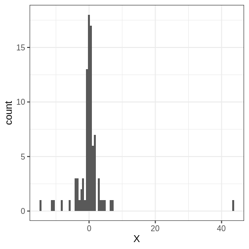
Posterior predictive check
The idea of posterior predictive checking is to use the posterior predictive distribution to simulate a replicate data set and compare it to the observed data. The reasoning behind this approach is that if the model is a good fit, then data generated from the model should look similar the observed data. Any qualitative discrepancies between the simulated and observed data can imply shortcomings in the model that do not match the properties of the data or the domain.
Comparison between simulated and actual data can be done in different ways. Visual comparison is an option but a more rigorous approach is to compute the posterior predictive p-value (\(ppp\)), which measures how well the model can reproduce the observed data. Computing the \(ppp\) requires specifying a statistic whose value is compared between the posterior predictive and the observed data.
The posterior predictive check, utilizing \(ppp\), can be formulated in the following points:
- Generate replicate data: Use the posterior predictive distribution to simulate new datasets \(X^{rep}\) with characteristics matching the observed data. In our example, this amounts to generating a replication of data with sample size \(N=88\) for each posterior sample.
- Choose test quantity \(T(X)\): Choose an aspect of the data that you wish to check. We’ll use the maximum value of the data as the test quantity and compute it for the observed data and for each replication: \(X^{rep}\).
- Compute \(ppp\): The posterior predictive p-value is defined as the probability \(Pr(T(X^{rep}) \geq T(X) | X)\), that is the probability that the predictions produce test quantities at least as extreme as those found in the data. Using samples, it is computed as the proportion of replicate data sets with \(T\) not smaller than that of \(T(X)\).
The smaller the \(ppp\)-value, the bigger the evidence that the model doesn’t capture the properties of the data.
Next, we will perform a posterior predictive check on the example data and compare the results for the normal and Cauchy models.
Normal model
We’ll use a basic Stan program for the normal model and produce the
replicate data in the generated quantities block. Notice that
X_rep is a vector with length equal to the sample size
\(N\). The values of X_rep
are generated in a loop using the random number generator
normal_rng. Notice that a single posterior value of \((\mu, \sigma)\) is used for each evaluation
of the generated quantities block; one posterior value is used to
generate one realization of \(X^{rep}\).
STAN
data {
  int<lower=0> N;
  vector[N] X;
}
parameters {
  real<lower=0> sigma;
  real mu;
}
model {
  X ~ normal(mu, sigma);

  mu ~ normal(0, 1);
  sigma ~ gamma(2, 1);
}

generated quantities {
  vector[N] X_rep;

  for(i in 1:N) {
    X_rep[i] = normal_rng(mu, sigma);
  }
}
Let’s fit model and extract the replicates.
R
# Fit
normal_fit <- sampling(normal_model,
                       list(N = N, X = df$X),
                       refresh = 0)

# Extract
X_rep <- rstan::extract(normal_fit, "X_rep")[[1]] %>%
  data.frame() %>%
  mutate(sample = 1:nrow(.))
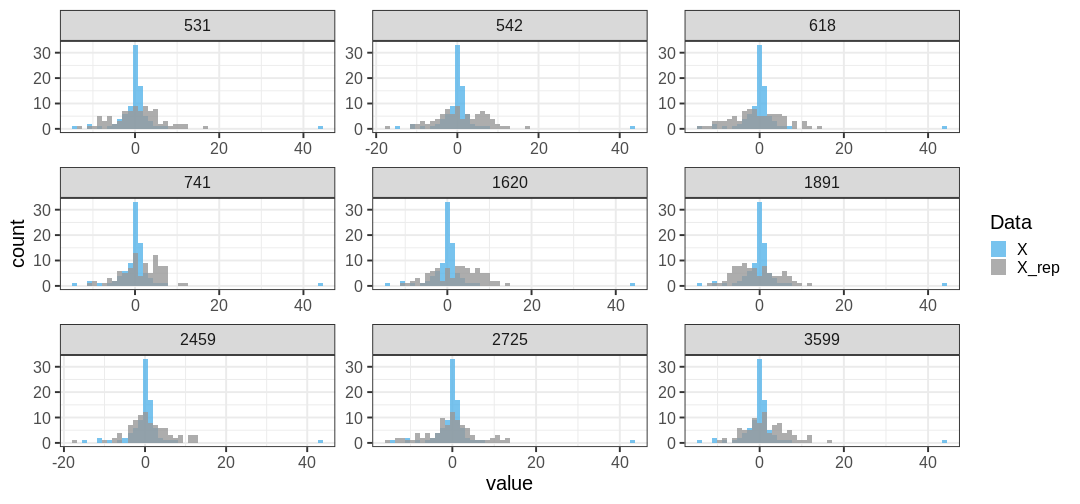
Below is a comparison of 9 realizations of \(X^{rep}\) (blue) against the data (grey; the panel titles correspond to MCMC sample numbers). It is evident that the tail properties are different between \(X^{rep}\) and \(X\), and this discrepancy indicates an issue with the model choice.
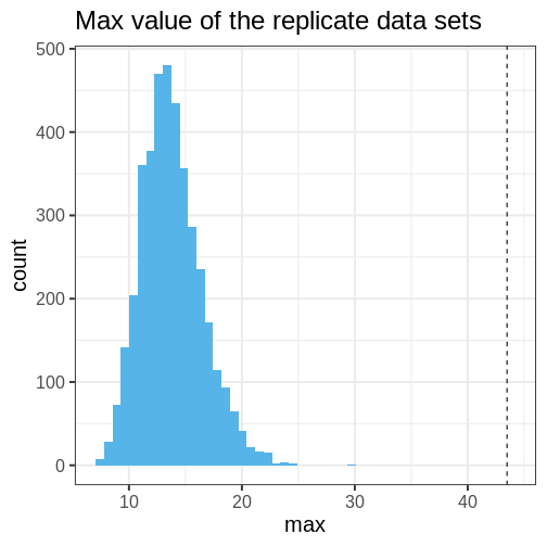
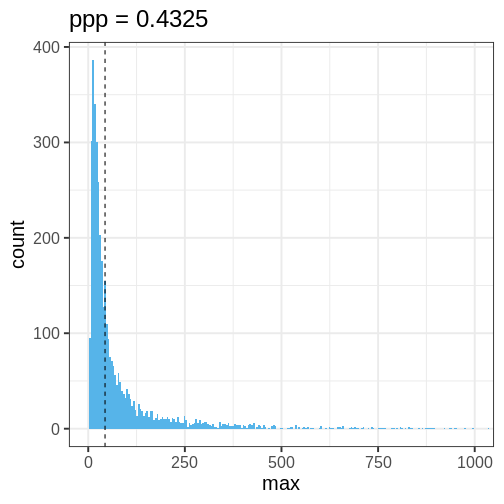
Let’s quantify this discrepancy by computing the \(ppp\) using the maximum of the data as a test statistic. The maximum of the original data is max(\(X\)) = 43.481. The \(ppp\), or the proportion of posterior prediction with a maximal value at least as large as this, is \(ppp =\) 1.
This means that the chosen statistic \(T\) is at least as large as in the data in 0% of the replications. This indicates strong evidence that the normal model is a poor choice for the data.
The following histogram displays \(T(X) = \max(X)\) (vertical line) against the distribution of \(T(X^{rep})\).
Cauchy model
Let’s do an identical analysis using the Cauchy model.
The results are generated with code that is essentially copy-pasted from above, with a minor distinction in the Stan program.
STAN
data {
int<lower=0> N;
vector[N] X;
}
parameters {
// Scale
real<lower=0> sigma;
// location
real mu;
}
model {
// location = mu and scale = sigma
X ~ cauchy(mu, sigma);
mu ~ normal(0, 1);
sigma ~ gamma(2, 1);
}
generated quantities {
vector[N] X_rep;
for(i in 1:N) {
X_rep[i] = cauchy_rng(mu, sigma);
}
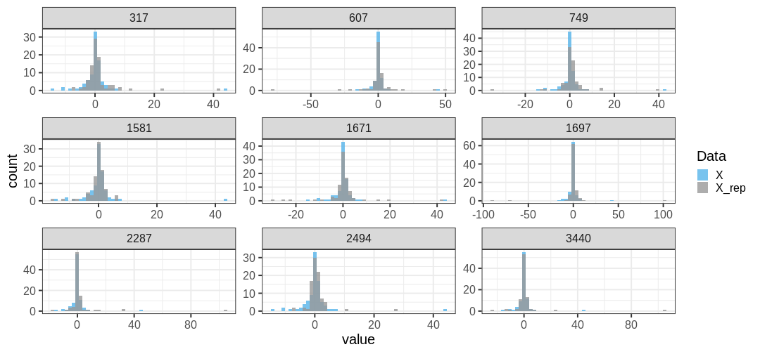
}A comparison of data \(X\) and \(X^{rep}\) from the Cauchy model reveals little discrepancy between the posterior predictions and the data. The distributions appear to closely match around 0, and the replicates contain extreme values similarly to the data.
The maximum value observed in the data is similar to those from replicate sets. Additionally, \(ppp\) is large, indicating no issues with the suitability of the model for the data. The conclusion drawn from this posterior predictive analysis is that the Cauchy distribution provides a better description of the data compared to the normal distribution.
Information criteria
Information criteria are statistics used for model comparison within both Bayesian and classical frequentist frameworks. These criteria provide a means to compare the relative suitability of a model to data by estimating out-of-sample predictive accuracy while simultaneously taking model complexity into account.
The Widely Applicable Information Criterion (WAIC) is an example of an information criteria developed within the Bayesian framework. WAIC is computed using the log pointwise predictive density (lppd) and the available data. Since the same data is used in both tasks, lppd may be an overly confident estimate of the predictive capability. To take this into account, a penalization term \(p_{WAIC}\) is included:
\[WAIC = -2(\text{lppd} - p_{WAIC}).\]
The log pointwise predictive density is computed as ${i=1}^N ( {s=1}^S p(X_i | ^s)), $, where \(X_i, \,i=1,\ldots,N\) are data points and \(S\) the number of posterior samples. The penalization term \(p_{WAIC} = \sum_{i=1}^N \text{Var}(\log p(y_i | \theta^s))\) measures the effective number of parameters (although this may not be apparent from the formula). Because the definition contains a negative of the difference \(\text{lppd} - p_{WAIC}\), lower WAIC values imply better fit.
Let’s use the WAIC to compare the normal and Cauchy models. First we’ll need to fit both models on the data using the Stan programs presented above.
R
stan_data <- list(N = N, X = df$X)

# Fit
normal_fit <- sampling(normal_model, stan_data,
                       refresh = 0)
cauchy_fit <- sampling(cauchy_model, stan_data,
                       refresh = 0)


# Extract samples
normal_samples <- rstan::extract(normal_fit, c("mu", "sigma")) %>% data.frame
cauchy_samples <- rstan::extract(cauchy_fit, c("mu", "sigma")) %>% data.frame
Then we can write a function to compute lppd and the penalization, and combine these into WAIC
R
WAIC <- function(samples, data, model){

  # Loop over data points
  pp_dens <- lapply(1:length(data), function(i) {

    my_x <- data[i]

    # Loop over posterior samples
    point_pp_dens <- lapply(1:nrow(samples), function(S) {

      my_mu <- samples[S, "mu"]
      my_sigma <- samples[S, "sigma"]

      if(model == "normal") {
        # Model: y ~ normal(mu, sigma)
        dnorm(x = my_x,
              mean = my_mu,
              sd = my_sigma)
      } else if(model == "cauchy") {
        # Model: y ~ Cauchy(mu, sigma)
        dcauchy(x = my_x,
                location = my_mu,
                scale = my_sigma)
      }

    }) %>%
      unlist()

    return(point_pp_dens)

  }) %>%
    do.call(rbind, .)


  # See BDA3 p.169
  lppd <- apply(X = pp_dens,
                MARGIN = 1,
                FUN = function(x) log(mean(x))) %>%
    sum

  # See BDA3 p.173
  bias <- apply(X = pp_dens,
                MARGIN = 1,
                FUN = function(x) var(log(x))) %>%
    sum

  # WAIC
  waic = -2*(lppd - bias)

  return(waic)
}
Applying this function to the posterior samples, we’ll obtain a lower value for the Cauchy model, implying a better fit to the data. This is in line with the posterior predictive check performed above.
R
WAIC(normal_samples, df$X, model = "normal")
OUTPUT
[1] 582.6821R
WAIC(cauchy_samples, df$X, model = "cauchy")
OUTPUT
[1] 413.7336Bayesian cross-validation
The final approach we take to model comparison in cross-validation.
Cross-validation is a technique that estimates how well a model predicts previously unseen data by using fits of the model to a subset of the data to predict the rest of the data.
Performing cross-validation entails defining the amount of leave-out data. The larger the proportion of the data used for model training, the better the accuracy. However, increasing size of training data leads to having to fit a larger number of models. In the extreme case, when each data point is left out individually, we talk about leave-one-out cross-validation and need \(n\) data partition, and fits.
In general in machine learning and statistics, the prediction made on the test set need to be evaluated. There are different metrics. Here, we will use log predictive density as a metric and take the sum over the different fits as the representation of predictive accuracy. Then we will compare this to the predictive densities computed using the model fit with all the data. This difference represents the effective number of parameters that can be used for comparing models.
\[p_{\text{loo-cv}} = \text{lppd} - \text{lppd}_\text{loo-cv},\] where \(\text{lppd}_\text{loo-cv}\) is the sum of the log predictive densities of individual data points evaluated based on the model trained without the particular data point.
Let’s first write a helper function that computes the log predictive density for a point, given posterior samples and the model.
R
# Get log predictive density for a point x,
# given data X and posterior samples
# See BDA3 p.175
get_lpd <- function(x, samples, model) {

  # Loop over posterior samples
  pp_dens <- lapply(1:nrow(samples), function(S) {

    if(model == "normal") {
      # Normal(x | mu, sigma^2)
      dnorm(x = x,
            mean = samples[S, "mu"],
            sd = samples[S, "sigma"])
    } else if (model == "cauchy") {
      # Cauchy(x | location = mu, scale = sigma^2)
      dcauchy(x = x,
              location = samples[S, "mu"],
              scale = samples[S, "sigma"])
    }

  }) %>%
    unlist()

  lpd <- log(mean(pp_dens))

  return(lpd)
}
Now we can perform cross-validation for the normal and Cauchy models:
R
# Loop over data partitions
normal_loo_lpds <- lapply(1:N, function(i) {

  # Training set
  my_X <- X[-i]

  # Test set
  my_x <- X[i]

  # Fit model
  my_normal_fit <- sampling(normal_model,
                            list(N = length(my_X),
                                 X = my_X),
                            refresh = 0 # omit output
                            )

  # Get data
  my_samples <- rstan::extract(my_normal_fit, c("mu", "sigma")) %>%
    do.call(cbind, .) %>%
    set_colnames(c("mu", "sigma"))

  # Get lpd
  my_lpd <- get_lpd(my_x, my_samples, "normal")

  data.frame(i, lpd = my_lpd, model = "normal_loo")

}) %>%
  do.call(rbind, .)

# Predictive density for data points using full data in training
normal_full_lpd <- lapply(1, function(dummy) {

  # Fit model
  my_normal_fit <- sampling(normal_model,
                            list(N = length(X),
                                 X = X),
                            refresh = 0)

  # Get data
  my_samples <- rstan::extract(my_normal_fit, c("mu", "sigma")) %>%
    do.call(cbind, .) %>%
    set_colnames(c("mu", "sigma"))

  # Compute lpds
  lpds <- lapply(1:N, function(i) {

    my_lpd <- get_lpd(X[i], my_samples, "normal")

    data.frame(i, lpd = my_lpd, model = "normal")
  }) %>% do.call(rbind, .)

  return(lpds)
}) %>%
  do.call(rbind, .)


# Same for Cauchy:
cauchy_loo_lpds <- lapply(1:N, function(i) {

  # Subset data
  my_X <- X[-i]
  my_x <- X[i]

  # Fit model
  my_normal_fit <- sampling(cauchy_model,
                            list(N = length(my_X),
                                 X = my_X),
                            refresh = 0)

  # Get data
  my_samples <- rstan::extract(my_normal_fit, c("mu", "sigma")) %>%
    do.call(cbind, .) %>%
    set_colnames(c("mu", "sigma"))

  # Get lpd
  my_lpd <- get_lpd(my_x, my_samples, "cauchy")

  data.frame(i, lpd = my_lpd, model = "cauchy_loo")

}) %>%
  do.call(rbind, .)

cauchy_full_lpd <- lapply(1, function(dummy) {

  # Fit model
  my_cachy_fit <- sampling(cauchy_model,
                           list(N = length(X),
                                X = X),
                           refresh = 0)

  # Get data
  my_samples <- rstan::extract(my_cachy_fit, c("mu", "sigma")) %>%
    do.call(cbind, .) %>%
    set_colnames(c("mu", "sigma"))

  # Compute lpds
  lpds <- lapply(1:N, function(i) {

    my_lpd <- get_lpd(X[i], my_samples, "cauchy")

    data.frame(i, lpd = my_lpd, model = "cauchy")
  }) %>% do.call(rbind, .)

  return(lpds)
}) %>%
  do.call(rbind, .)
Let’s combine the computed log densities, and compute model-wise sums
R
# Combine
lpds <- rbind(normal_loo_lpds,
              normal_full_lpd,
              cauchy_loo_lpds,
              cauchy_full_lpd)

lpd_summary <- lpds %>%
  group_by(model) %>%
  summarize(lppd = sum(lpd))
Finally, we can compute the estimated of the effective number of parameters. As with WAIC, smaller values imply better suitability. In line with the posterior predictive check and WAIC, we see that, again, the Cauchy distribution gives a better description of the data that the normal model.
R
# Effective number of parameters
p_loo_cv_normal <- lpd_summary[lpd_summary$model == "normal", "lppd"] - lpd_summary[lpd_summary$model == "normal_loo", "lppd"]
p_loo_cv_cauchy <- lpd_summary[lpd_summary$model == "cauchy", "lppd"] - lpd_summary[lpd_summary$model == "cauchy_loo", "lppd"]


paste0("Effective number of parameters, normal = ", p_loo_cv_normal)
OUTPUT
[1] "Effective number of parameters, normal = 33.7059542565819"R
paste0("Effective number of parameters, cauchy = ", p_loo_cv_cauchy)
OUTPUT
[1] "Effective number of parameters, cauchy = 1.903135942788"Reading
Statistical Rethinking: Ch. 7
BDA3: p.143: 6.3 Posterior predictive checking
PSIS-loo