t-tests in practice
Last updated on 2026-03-24 | Edit this page
Estimated time: 0 minutes
Overview
Questions
- How are t-tests used in practice?
Objectives
t-tests in Practice
Introduction
We will now demonstrate how to obtain a p-value in practice. We begin by loading experimental data and walking you through the steps used to form a t-statistic and compute a p-value. We can perform this task with just a few lines of code (go to the end of this section to see them). However, to understand the concepts, we will construct a t-statistic from “scratch”.
Read in and prepare data
We start by reading in the data. A first important step is to identify which rows are associated with treatment and control, and to compute the difference in mean.
R
fWeights <- read.csv(file = "./data/femaleMiceWeights.csv") # we read this data in earlier
control <- filter(fWeights, Diet=="chow") %>%
  select(Bodyweight) %>%
  unlist
treatment <- filter(fWeights, Diet=="hf") %>%
  select(Bodyweight) %>%
  unlist
diff <- mean(treatment) - mean(control)
print(diff)
OUTPUT
[1] 3.020833We are asked to report a p-value. What do we do? We learned that
diff, referred to as the observed effect size, is
a random variable. We also learned that under the null hypothesis, the
mean of the distribution of diff is 0. What about the
standard error? We also learned that the standard error of this random
variable is the population standard deviation divided by the square root
of the sample size:
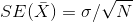
We use the sample standard deviation as an estimate of the population
standard deviation. In R, we simply use the sd function and
the SE is:
R
sd(control)/sqrt(length(control))
OUTPUT
[1] 0.8725323This is the SE of the sample average, but we actually want the SE of
diff. We saw how statistical theory tells us that the
variance of the difference of two random variables is the sum of its
variances, so we compute the variance and take the square root:
R
se <- sqrt(
  var(treatment)/length(treatment) +
  var(control)/length(control)
  )
Statistical theory tells us that if we divide a random variable by its SE, we get a new random variable with an SE of 1.
R
tstat <- diff/se
This ratio is what we call the t-statistic. It’s the ratio of two random variables and thus a random variable. Once we know the distribution of this random variable, we can then easily compute a p-value.
As explained in the previous section, the CLT tells us that for large
sample sizes, both sample averages mean(treatment) and
mean(control) are normal. Statistical theory tells us that
the difference of two normally distributed random variables is again
normal, so CLT tells us that tstat is approximately normal
with mean 0 (the null hypothesis) and SD 1 (we divided by its SE).
So now to calculate a p-value all we need to do is ask: how often
does a normally distributed random variable exceed diff? R
has a built-in function, pnorm, to answer this specific
question. pnorm(a) returns the probability that a random
variable following the standard normal distribution falls below
a. To obtain the probability that it is larger than
a, we simply use 1-pnorm(a). We want to know
the probability of seeing something as extreme as diff:
either smaller (more negative) than -abs(diff) or larger
than abs(diff). We call these two regions “tails” and
calculate their size:
R
righttail <- 1 - pnorm(abs(tstat))
lefttail <- pnorm(-abs(tstat))
pval <- lefttail + righttail
print(pval)
OUTPUT
[1] 0.0398622In this case, the p-value is smaller than 0.05 and using the conventional cutoff of 0.05, we would call the difference statistically significant.
Now there is a problem. CLT works for large samples, but is 12 large enough? A rule of thumb for CLT is that 30 is a large enough sample size (but this is just a rule of thumb). The p-value we computed is only a valid approximation if the assumptions hold, which do not seem to be the case here. However, there is another option other than using CLT.
The t-distribution in Practice
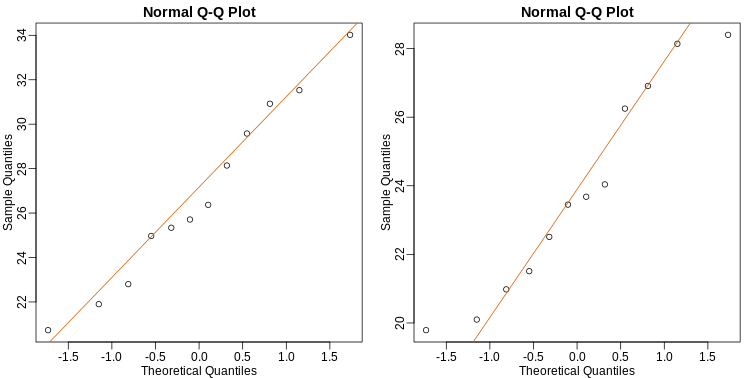
As described earlier, statistical theory offers another useful result. If the distribution of the population is normal, then we can work out the exact distribution of the t-statistic without the need for the CLT. This is a big “if” given that, with small samples, it is hard to check if the population is normal. But for something like weight, we suspect that the population distribution is likely well approximated by normal and that we can use this approximation. Furthermore, we can look at a qq-plot for the samples. This shows that the approximation is at least close:
R
library(rafalib)
mypar(1,2)
qqnorm(treatment)
qqline(treatment, col=2)
qqnorm(control)
qqline(control, col=2)
If we use this approximation, then statistical theory tells us that
the distribution of the random variable tstat follows a
t-distribution. This is a much more complicated distribution than the
normal. The t-distribution has a location parameter like the normal and
another parameter called degrees of freedom. R has a nice
function that actually computes everything for us.
R
t.test(treatment, control)
OUTPUT
	Welch Two Sample t-test

data:  treatment and control
t = 2.0552, df = 20.236, p-value = 0.053
alternative hypothesis: true difference in means is not equal to 0
95 percent confidence interval:
 -0.04296563  6.08463229
sample estimates:
mean of x mean of y
 26.83417  23.81333
To see just the p-value, we can use the $ extractor:
R
result <- t.test(treatment,control)
result$p.value
OUTPUT
[1] 0.05299888The p-value is slightly bigger now. This is to be expected because
our CLT approximation considered the denominator of tstat
practically fixed (with large samples it practically is), while the
t-distribution approximation takes into account that the denominator
(the standard error of the difference) is a random variable. The smaller
the sample size, the more the denominator varies.
It may be confusing that one approximation gave us one p-value and another gave us another, because we expect there to be just one answer. However, this is not uncommon in data analysis. We used different assumptions, different approximations, and therefore we obtained different results.
Later, in the power calculation section, we will describe type I and type II errors. As a preview, we will point out that the test based on the CLT approximation is more likely to incorrectly reject the null hypothesis (a false positive), while the t-distribution is more likely to incorrectly accept the null hypothesis (false negative).
Running the t-test in practice
Now that we have gone over the concepts, we can show the relatively simple code that one would use to actually compute a t-test:
R
control <- filter(fWeights, Diet=="chow") %>%
  select(Bodyweight) %>%
  unlist
treatment <- filter(fWeights, Diet=="hf") %>%
  select(Bodyweight) %>%
  unlist
t.test(treatment, control)
OUTPUT
	Welch Two Sample t-test

data:  treatment and control
t = 2.0552, df = 20.236, p-value = 0.053
alternative hypothesis: true difference in means is not equal to 0
95 percent confidence interval:
 -0.04296563  6.08463229
sample estimates:
mean of x mean of y
 26.83417  23.81333
The arguments to t.test can be of type
data.frame and thus we do not need to unlist them into numeric
objects.
- .
- .
- .
- .