Introducing Scikit Learn

Overview

Teaching: 15 min
Exercises: 20 min

Questions

• How can I use scikit-learn to process data?

Objectives

• Recall that scikit-learn has built in linear regression functions.

• Measure the error between a regression model and real data.

• Apply scikit-learn’s linear regression to create a model.

• Analyse and assess the accuracy of a linear model using scikit-learn’s metrics library.

• Understand that more complex models can be built with non-linear equations.

• Apply scikit-learn’s polynomial modelling to non-linear data.

SciKit Learn (also known as sklearn) is an open source machine learning library for Python which has a very wide range of machine learning algorithms. It makes it very easy for a Python programmer to use machine learning techniques without having to implement them.

Linear Regression with scikit-learn

Lets adapt our linear regression program to use scikit-learn instead of our own regression function. We can go and remove the least_squares and measure_error functions from our code. We’ll save this under a different filename to the original linear regression code so that we can compare the answers of the two, they should be identical.

First lets add the import for sklearn, we’re also going to need the numpy library so we’ll import that too:

import numpy as np
import sklearn.linear_model as skl_lin

Now lets replace the calculation with our own least_squares function with the one from scikit-learn. The scikit-learn regression function is much more capable than the simple one we wrote earlier and is designed for datasets where multiple parameters are used, its expecting to be given multi-demnsional arrays data. To get it to accept single dimension data such as we have we need to convert the array to a numpy one and use numpy’s reshape function. The resulting data is also designed to show us multiple coefficients and intercepts, so these values will be arrays, since we’ve just got one parameter we can just grab the first item from each of these arrays. Instead of manually calculating the results we can now use scikit-learn’s predict function. Finally lets calculate the error. scikit-learn doesn’t provide a root mean squared error function, but it does provide a mean squared error function. We can calculate the root mean squared error simply by taking the square root of the output of this function. The mean_squared_error function is part of the scikit-learn metrics module, so we’ll have to add that to our imports at the top of the file:

import sklearn.metrics as skl_metrics

Lets go ahead and change the process_data function for life expectancy to use scikit-learn’s LinearRegression function instead of our own version.

import pandas as pd
import math
def process_life_expectancy_data(filename, country, min_date, max_date):
    df = pd.read_csv(filename, index_col="Life expectancy")

    # get the life expectancy for the specified country/dates
    # we have to convert the dates to strings as pandas treats them that way
    life_expectancy = df.loc[country, str(min_date):str(max_date)]
    x_data = list(range(min_date, max_date + 1))

    x_data_arr = np.array(x_data).reshape(-1, 1)
    life_exp_arr = np.array(life_expectancy).reshape(-1, 1)

    regression = skl_lin.LinearRegression().fit(x_data_arr, life_exp_arr)

    m = regression.coef_[0][0]
    c = regression.intercept_[0]

    # old manual version
    #linear_data = calculate_linear(x_data, m, c)

    # new scikit learn version
    linear_data = regression.predict(x_data_arr)

    # old manual version
    #error = measure_error(life_expectancy, linear_data)

    # new scikit learn version
    error = math.sqrt(skl_metrics.mean_squared_error(life_exp_arr, linear_data))
    print("error=", error)

    # uncomment to make the graph
    #make_graph(life_exp, gdp, linear_data)

process_life_expectancy_data("../data/gapminder-life-expectancy.csv",
                             "United Kingdom", 1950, 2016)

Now if we go ahead and run the new program we should get the same answers and same graph as before.

Comparing the Scikit learn and our own linear regression implementations.

Adjust both the original program (using our own linear regression implementation) and the sklearn version to calculate the life expectancy for Germany between 1950 and 2000. What are the values (m and c) of linear equation linking date and life expectancy? Are they the same in both?

Solution

process_life_expectancy_data("../data/gapminder-life-expectancy.csv", "Germany", 1950, 2000)

m= 0.212219909502 c= -346.784909502 They should be identical

Predicting Life Expectancy

Use the linear equation you’ve just created to predict life expectancy in Germany for every year between 2001 and 2016. How accurate are your answers? If you worked for a pension scheme would you trust your answers to predict the future costs for paying pensioners?

Solution

for x in range(2001,2017):
    print(x,0.212219909502 * x - 346.784909502)

Predicted answers:

2001 77.86712941150199
2002 78.07934932100403
2003 78.29156923050601
2004 78.503789140008
2005 78.71600904951003
2006 78.92822895901202
2007 79.140448868514
2008 79.35266877801604
2009 79.56488868751802
2010 79.77710859702
2011 79.98932850652199
2012 80.20154841602402
2013 80.41376832552601
2014 80.62598823502799
2015 80.83820814453003
2016 81.05042805403201

Compare with the real values:

df = pd.read_csv('../data/gapminder-life-expectancy.csv',index_col="Life expectancy")
for x in range(2001,2017):
    y = 0.215621719457 * x - 351.935837103
    real = df.loc['Germany', str(x)]
    print(x, "Predicted", y, "Real", real, "Difference", y-real)

2001 Predicted 77.86712941150199 Real 78.4 Difference -0.532870588498
2002 Predicted 78.07934932100403 Real 78.6 Difference -0.520650678996
2003 Predicted 78.29156923050601 Real 78.8 Difference -0.508430769494
2004 Predicted 78.503789140008 Real 79.2 Difference -0.696210859992
2005 Predicted 78.71600904951003 Real 79.4 Difference -0.68399095049
2006 Predicted 78.92822895901202 Real 79.7 Difference -0.771771040988
2007 Predicted 79.140448868514 Real 79.9 Difference -0.759551131486
2008 Predicted 79.35266877801604 Real 80.0 Difference -0.647331221984
2009 Predicted 79.56488868751802 Real 80.1 Difference -0.535111312482
2010 Predicted 79.77710859702 Real 80.3 Difference -0.52289140298
2011 Predicted 79.98932850652199 Real 80.5 Difference -0.510671493478
2012 Predicted 80.20154841602402 Real 80.6 Difference -0.398451583976
2013 Predicted 80.41376832552601 Real 80.7 Difference -0.286231674474
2014 Predicted 80.62598823502799 Real 80.7 Difference -0.074011764972
2015 Predicted 80.83820814453003 Real 80.8 Difference 0.03820814453
2016 Predicted 81.05042805403201 Real 80.9 Difference 0.150428054032

Other types of regression

Linear regression obviously has its limits for working with data that isn’t linear. Scikit-learn has a number of other regression techniques which can be used on non-linear data. Some of these (such as isotonic regression) will only interpolate data in the range of the training data and can’t extrapolate beyond it. One non-linear technique that works with many types of data is polynomial regression. This creates a polynomial equation of the form y = a + bx + cx^2 + dx^3 etc. The more terms we add to the polynomial the more accurately we can model a system.

Scikit-learn includes a polynomial modelling tool as part of its pre-processing library which we’ll need to add to our list of imports.

import sklearn.preprocessing as skl_pre

Now lets modify the process_life_expectancy_data function to calculate the polynomial. This takes two parts, the first is to pre-process the data into polynomial form. We first call the PolynomialFeatures function with the parameter degree. The degree parameter controls how many components the polynomial will have, a polynomial of the form y = a + bx + cx^2 + dx^3 has 4 degrees. Typically a value between 5 and 10 is sufficient. We must then process the numpy array that we used for the X axis in the linear regression to convert it into a set of polynomial features.

This only gets us halfway to being able to create a model that we can use for predictions. To form the complete model we actually have to perform a linear regression on the polynomial model, but we’ll use the polynomial features as the X axis instead of the numpy array. The Y axis will still be the life expectancy numpy array that we used before. The resulting model can now be used to make some predictions like we did before using the predict function.

If we want to draw the line of best fit we can pass the polynomial features in as a parameter to predict() and this will generate the y values for the full range of our data. This can be plotted by passing it to make_graph in place of the linear data.

Finally we can make some predictions of future data. Lets create a list containing the date range we’d like to predict, as with other lists/arrays we’ve used we’ll have to reshape it to make scikit-learn work with it. Now lets use this list of dates to predict life expectancy using both our linear and polynomial models.

def process_life_expectancy_data_poly(filename, country, min_date, max_date):
    df = pd.read_csv(filename, index_col="Life expectancy")

    # get the life expectancy for the specified country/dates
    # we have to convert the dates to strings as pandas treats them that way
    life_expectancy = df.loc[country, str(min_date):str(max_date)]
    x_data = list(range(min_date, max_date + 1))

    x_data_arr = np.array(x_data).reshape(-1, 1)
    life_exp_arr = np.array(life_expectancy).reshape(-1, 1)

    polynomial_features = skl_pre.PolynomialFeatures(degree=5)
    x_poly = polynomial_features.fit_transform(x_data_arr)

    polynomial_model = skl_lin.LinearRegression().fit(x_poly, life_exp_arr)

    polynomial_data = polynomial_model.predict(x_poly)

    #make_graph(x_data, life_expectancy, polynomial_data)

    # make some predictions
    predictions_x = list(range(2011,2025))
    predictions_x_arr = np.array(predictions_x).reshape(-1, 1)

    predictions_polynomial = polynomial_model.predict(polynomial_features.fit_transform(predictions_x_arr))
    plt.plot(x_data, life_expectancy, label="Original Data")
    plt.plot(predictions_x, predictions_polynomial, label="Polynomial Prediction")
    plt.grid()
    plt.legend()
    plt.show()

To measure the error lets calculate the RMS error on both the linear and polynomial data.

def process_life_expectancy_data_poly(filename, country, min_date, max_date):
    df = pd.read_csv(filename, index_col="Life expectancy")

    # get the life expectancy for the specified country/dates
    # we have to convert the dates to strings as pandas treats them that way
    life_expectancy = df.loc[country, str(min_date):str(max_date)]
    x_data = list(range(min_date, max_date + 1))

    x_data_arr = np.array(x_data).reshape(-1, 1)
    life_exp_arr = np.array(life_expectancy).reshape(-1, 1)

    polynomial_features = skl_pre.PolynomialFeatures(degree=5)
    x_poly = polynomial_features.fit_transform(x_data_arr)

    polynomial_model = skl_lin.LinearRegression().fit(x_poly, life_exp_arr)

    polynomial_data = polynomial_model.predict(x_poly)

    polynomial_error = math.sqrt(
                   skl_metrics.mean_squared_error(life_exp_arr, polynomial_data))
    print("polynomial error is", polynomial_error)

process_life_expectancy_data_poly("../data/gapminder-life-expectancy.csv",
                             "United Kingdom", 1950, 2016)

process_life_expectancy_data("../data/gapminder-life-expectancy.csv",
                             "United Kingdom", 1950, 2016)

Exercise: Comparing linear and polynomial models

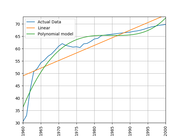
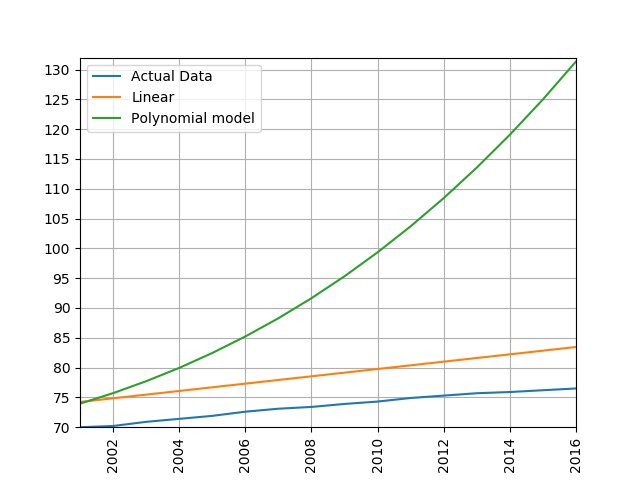
Train a linear and polynomial model on life expectancy data from China between 1960 and 2000. Then predict life expectancy from 2001 to 2016 using both methods. Compare their root mean squared errors, which is more accurate? Why do you think this model is the more accurate one?

Solution

modify the call to the process_life_expectancy_data

process_life_expectancy_data_poly("../data/gapminder-life-expectancy.csv", "China", 1960, 2000)

linear prediction error is 5.385162846665607 polynomial prediction error is 28.169167771983528 The linear model is more accurate, polynomial models often become wildly inaccurate beyond the range they were trained on. Look at the predicted life expectancies, the polynomial model predicts a life expectancy of 131 by 2016!

Key Points

• Scikit Learn is a Python library with lots of useful machine learning functions.

• Scikit Learn includes a linear regression function.

• It also includes a polynomial modelling function which is useful for modelling non-linear data.