Summary and Schedule
Introduction
This lesson introduces the core concepts of artificial neural networks through a practical application in healthcare: training a model to classify chest X-ray images.
You’ll learn how to:
- Load and visualize medical imaging data
- Prepare images for use in machine learning
- Build and train a convolutional neural network
- Evaluate model performance
- Explore explainability techniques using saliency maps
By the end of the lesson, you’ll have constructed a neural network capable of detecting pleural effusion in chest X-rays — a real-world example of how machine learning can assist clinical decision-making.
Prerequisites
You need to understand the basics of Python before tackling this lesson. The lesson sometimes references Jupyter Notebook although you can use any Python interpreter mentioned below in the setup instructions.
| Setup Instructions | Download files required for the lesson | |
| Duration: 00h 00m | 1. Introduction |
What kinds of conditions can be detected in chest X-rays? How does pleural effusion appear on a chest X-ray? How can chest X-ray data be used to train a machine learning model? |
| Duration: 00h 30m | 2. Visualisation |
How does a chest X-ray with pleural effusion differ from a normal
X-ray? How is an image represented and manipulated as a NumPy array? What steps are needed to prepare images for machine learning? |
| Duration: 01h 30m | 3. Data preparation |
Why do we divide data into training, validation, and test sets? What is data augmentation, and why is it useful for small datasets? How can random transformations help improve model performance? |
| Duration: 02h 30m | 4. Neural networks |
What is a neural network and how is it structured? What role do activation functions play in learning? What is the difference between dense and convolutional layers? Why are convolutional neural networks effective for image classification? |
| Duration: 03h 30m | 5. Training and evaluation |
How is a neural network trained to make better predictions? What do training loss and accuracy tell us? How do we evaluate a model’s performance on unseen data? |
| Duration: 04h 30m | 6. Explainability |
What is a saliency map, and how is it used to explain model
predictions? How do different explainability methods (e.g., GradCAM++ vs. ScoreCAM) compare? What are the limitations of saliency maps in practice? |
| Duration: 05h 30m | Finish |
The actual schedule may vary slightly depending on the topics and exercises chosen by the instructor.
Software Setup
This lesson is designed to be run on a personal computer. All of the software and data used in this lesson are freely available online, and instructions on how to obtain them are provided below.
Install Python
In this lesson, we will be using Python 3 with some of its most popular scientific libraries. Although one can install a plain-vanilla Python and all required libraries by hand, we recommend installing Anaconda, a Python distribution that comes with everything we need for the lesson. Detailed installation instructions for various operating systems can be found on The Carpentries template website for workshops and in Anaconda documentation.
Obtain lesson materials
The data that we are going to use for this project consists of 700 chest X-rays. These X-rays are a subset of the public NIH ChestX-ray dataset.
Xiaosong Wang, Yifan Peng, Le Lu, Zhiyong Lu, Mohammadhadi Bagheri, Ronald Summers, ChestX-ray8: Hospital-scale Chest X-ray Database and Benchmarks on Weakly-Supervised Classification and Localization of Common Thorax Diseases, IEEE CVPR, pp. 3462-3471, 2017
- Download chest_xrays.zip.
- Create a folder called
carpentries-ml-neuralon your Desktop. - Move downloaded files to
carpentries-ml-neural.
Launch Python interface
To start working with Python, we need to launch a program that will interpret and execute our Python commands. Below we list several options. If you don’t have a preference, proceed with the top option in the list that is available on your machine. Otherwise, you may use any interface you like.
Option A: Jupyter Notebook
A Jupyter Notebook provides a browser-based interface for working with Python. If you installed Anaconda, you can launch a notebook in two ways:
- Launch Anaconda Navigator. It might ask you if you’d like to send
anonymized usage information to Anaconda developers:
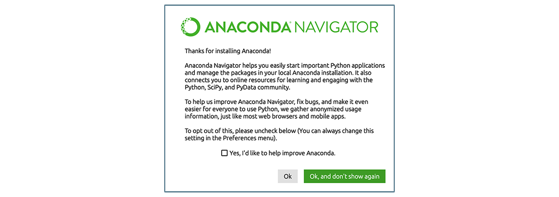 Make your choice and click “Ok,
and don’t show again” button.
Make your choice and click “Ok,
and don’t show again” button. - Find the “Notebook” tab and click on the “Launch” button:
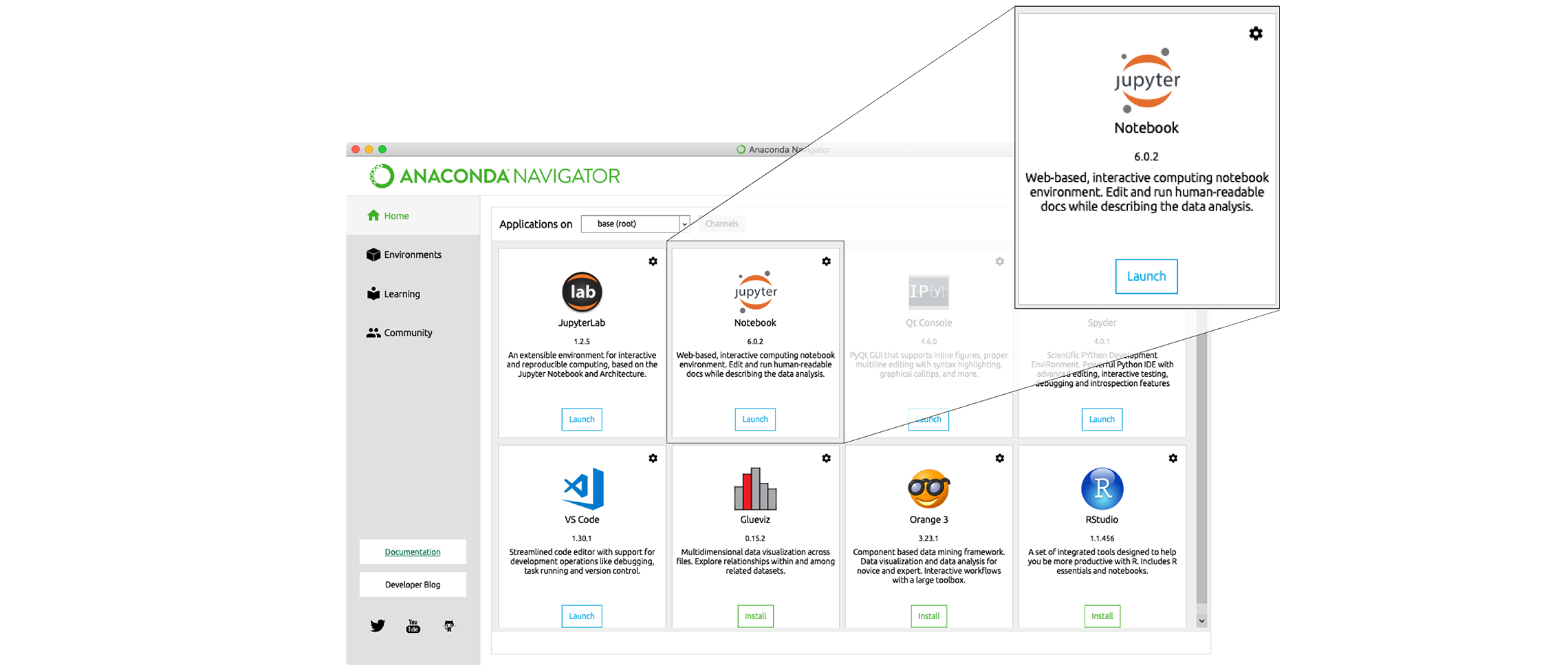 Anaconda will open a new
browser window or tab with a Notebook Dashboard showing you the contents
of your Home (or User) folder.
Anaconda will open a new
browser window or tab with a Notebook Dashboard showing you the contents
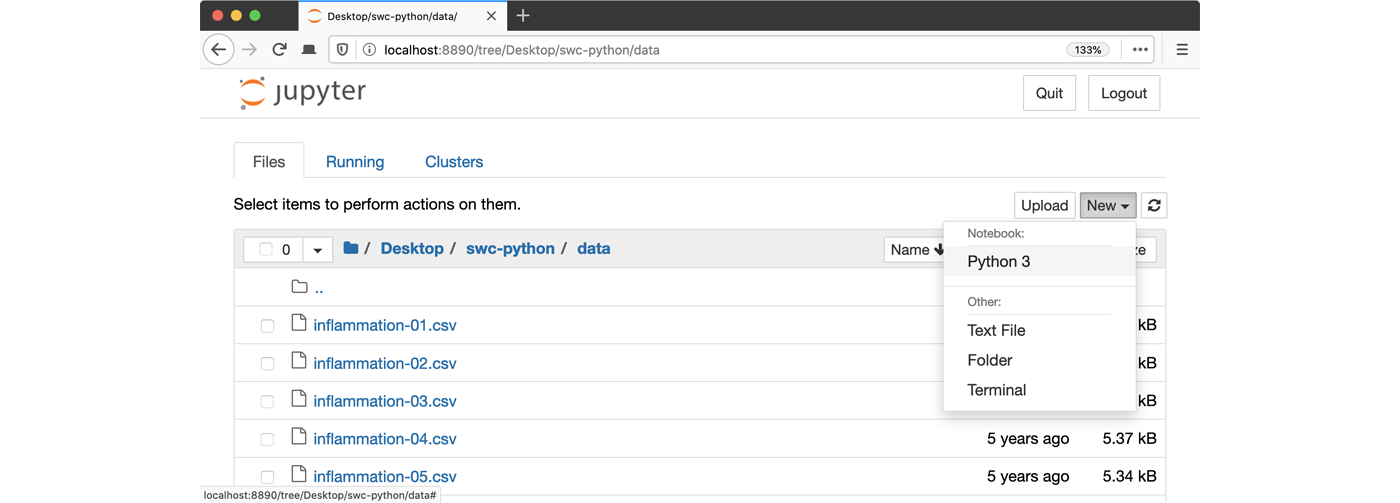
of your Home (or User) folder. - Navigate to the
datadirectory by clicking on the directory names leading to it:Desktop,swc-python, thendata: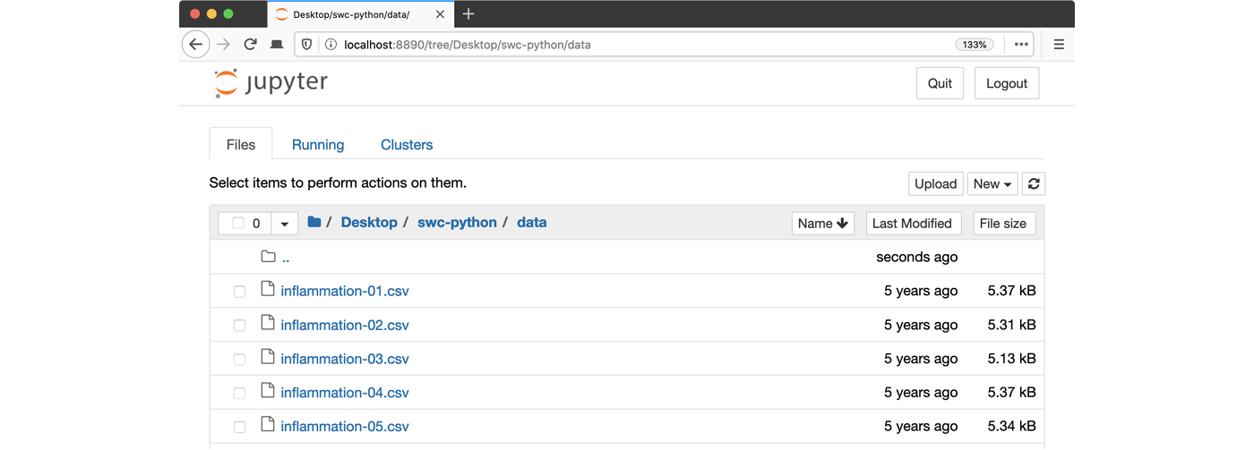
- Launch the notebook by clicking on the “New” button and then
selecting “Python 3”:
1. Navigate to the data directory:
If you’re using a Unix shell application, such as Terminal app in macOS, Console or Terminal in Linux, or Git Bash on Windows, execute the following command:
On Windows, you can use its native Command Prompt program. The
easiest way to start it up is pressing Windows Logo
Key+R, entering cmd, and hitting
Return. In the Command Prompt, use the following command to
navigate to the data folder:
cd /D %userprofile%\Desktop\swc-python\data2. Start Jupyter server
python -m notebook3. Launch the notebook by clicking on the “New” button on the right
and selecting “Python 3” from the drop-down menu: 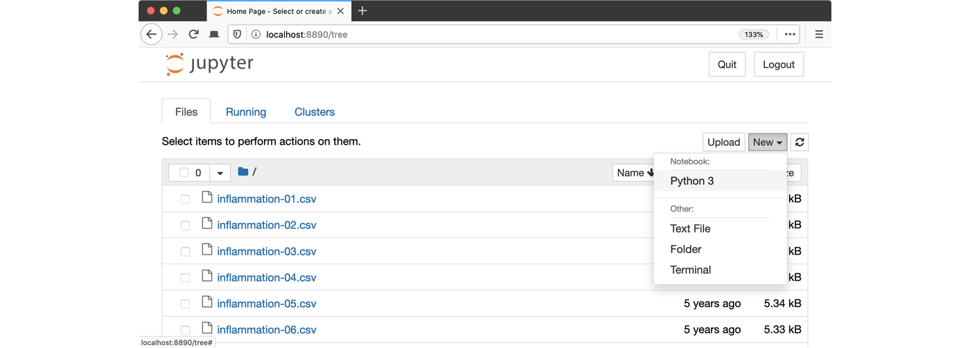
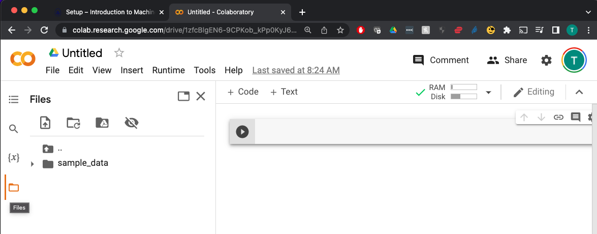
Option B: Cloud Notebook
Colaboratory, or “Colab”, is a cloud service that allows you to run a Jupyter-like Notebook in a web browser. To open a notebook, visit the Colaboratory website. You can upload your datasets using the “Files” panel on the left side of the page.