All Images
Welcome
Figure 1
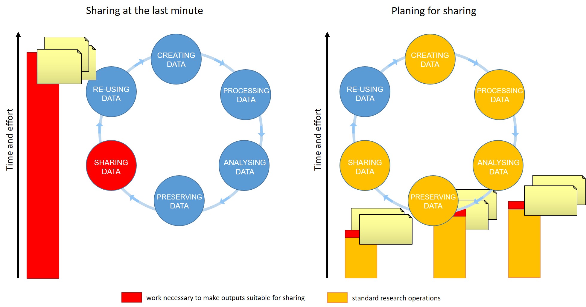 Figure credits:
Tomasz Zielinski and Andrés Romanowski
Figure credits:
Tomasz Zielinski and Andrés Romanowski
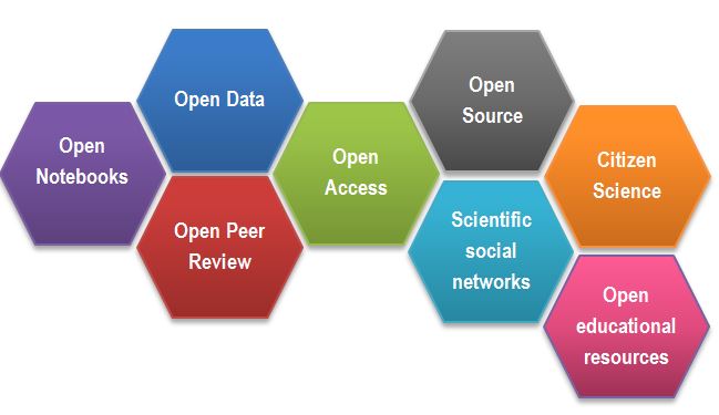
Introduction to Open Science
Figure 1
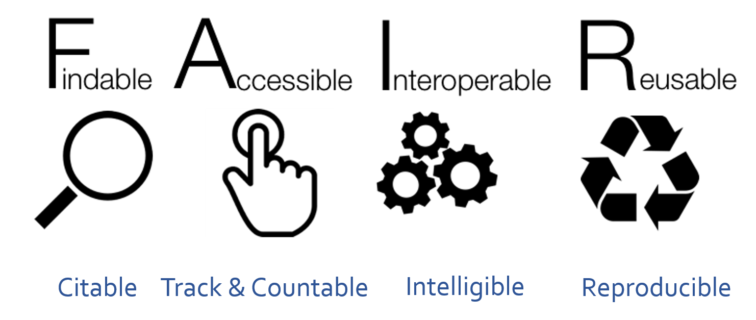
Being FAIR
Figure 1
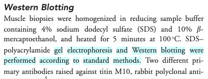
Figure 2
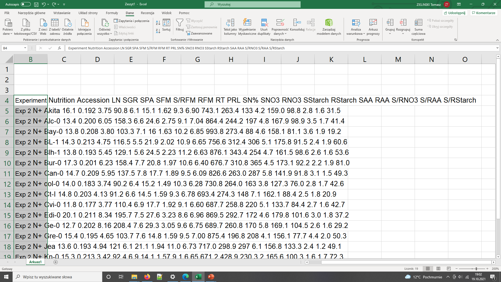
Data needs parsing after coping to Excel
The same data copied to Excel with polish locale has been converted to dates
Figure 3
 After SangyaPundir
Intellectual Property, Licensing and Openness
Introduction to metadata
Figure 1
 Figure credits: María Eugenia Goya
Figure 2
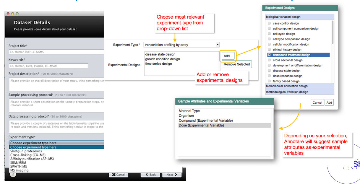
Here we have an excel spreadsheet that contains project metadata for
a made-up experiment of plant metabolites 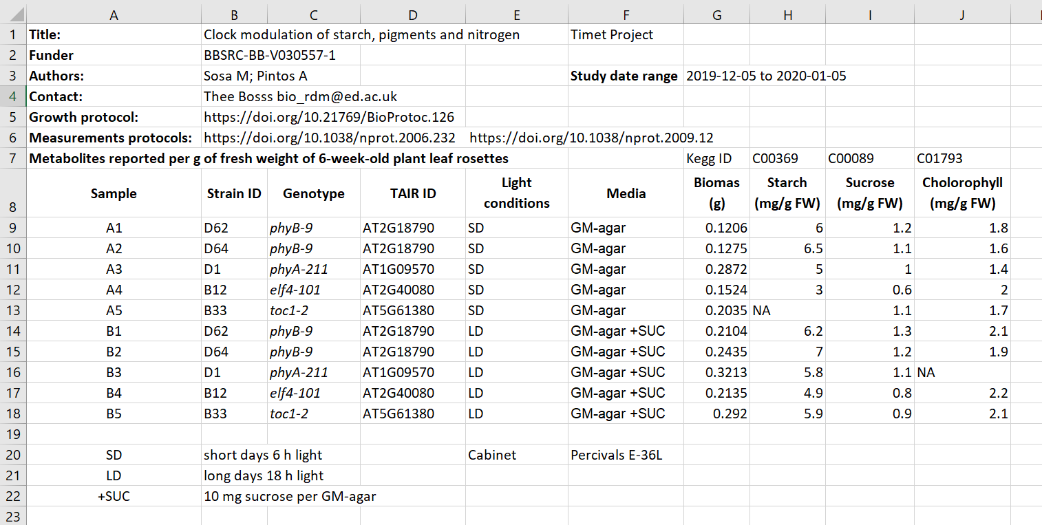 Figure credits: Tomasz
Zielinski and Andrés Romanowski
Figure credits: Tomasz
Zielinski and Andrés Romanowski
Figure 3
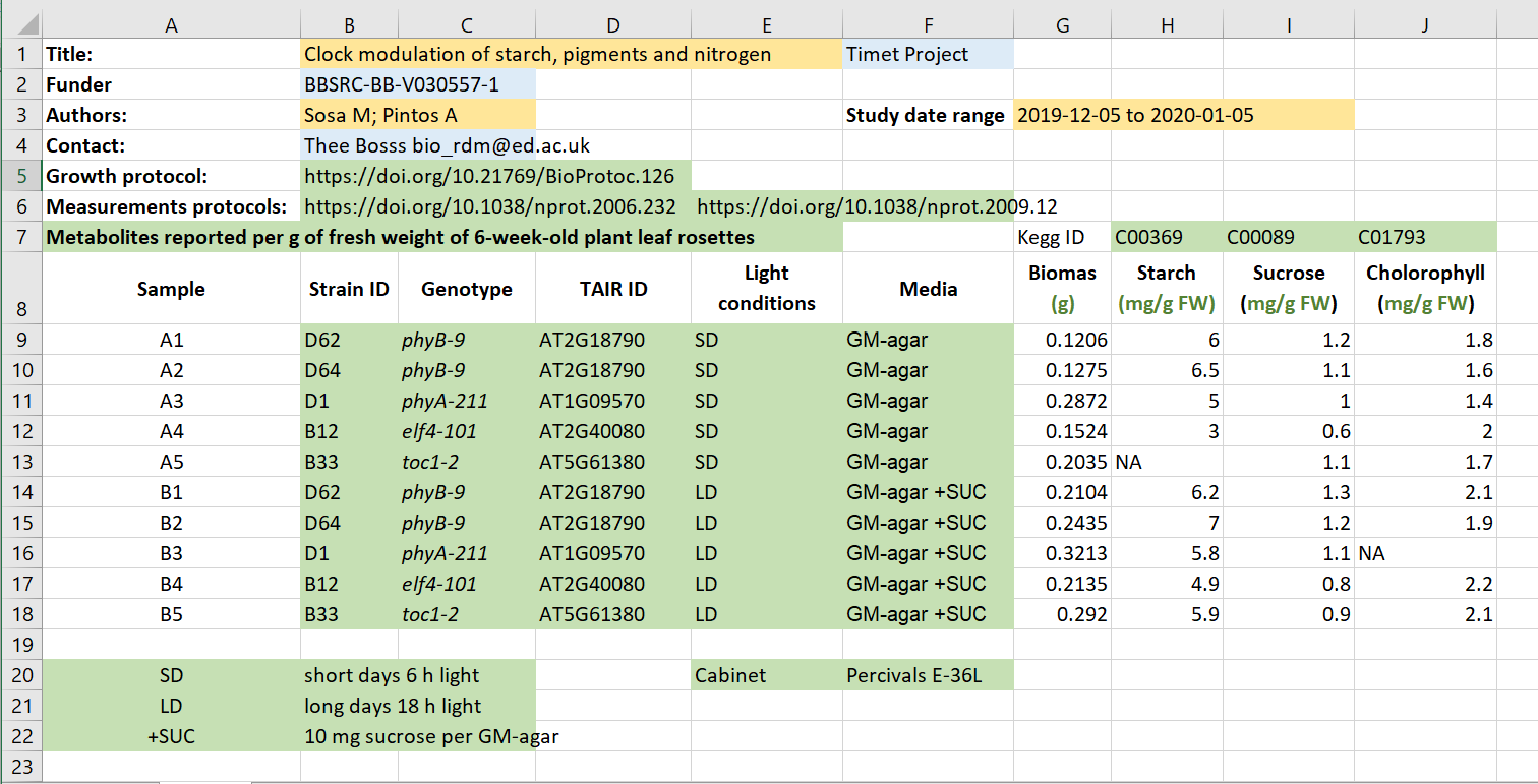 Figure credits: Tomasz Zielinski
and Andrés Romanowski
Figure credits: Tomasz Zielinski
and Andrés Romanowski
Being precise
Figure 1
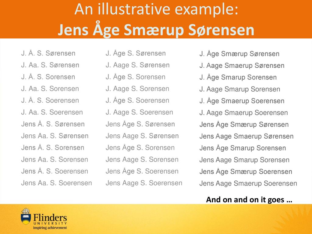
Figure 2
The second metadata example (the Excel table): contains two other
types of public IDs.Figure credits: Tomasz
Zielinski and Andrés Romanowski
Figure 3
 Example of graphical user
interfaces with controlled vocabularies
Example of graphical user
interfaces with controlled vocabularies
Figure 4
(Meta)data in Excel
Figure 1
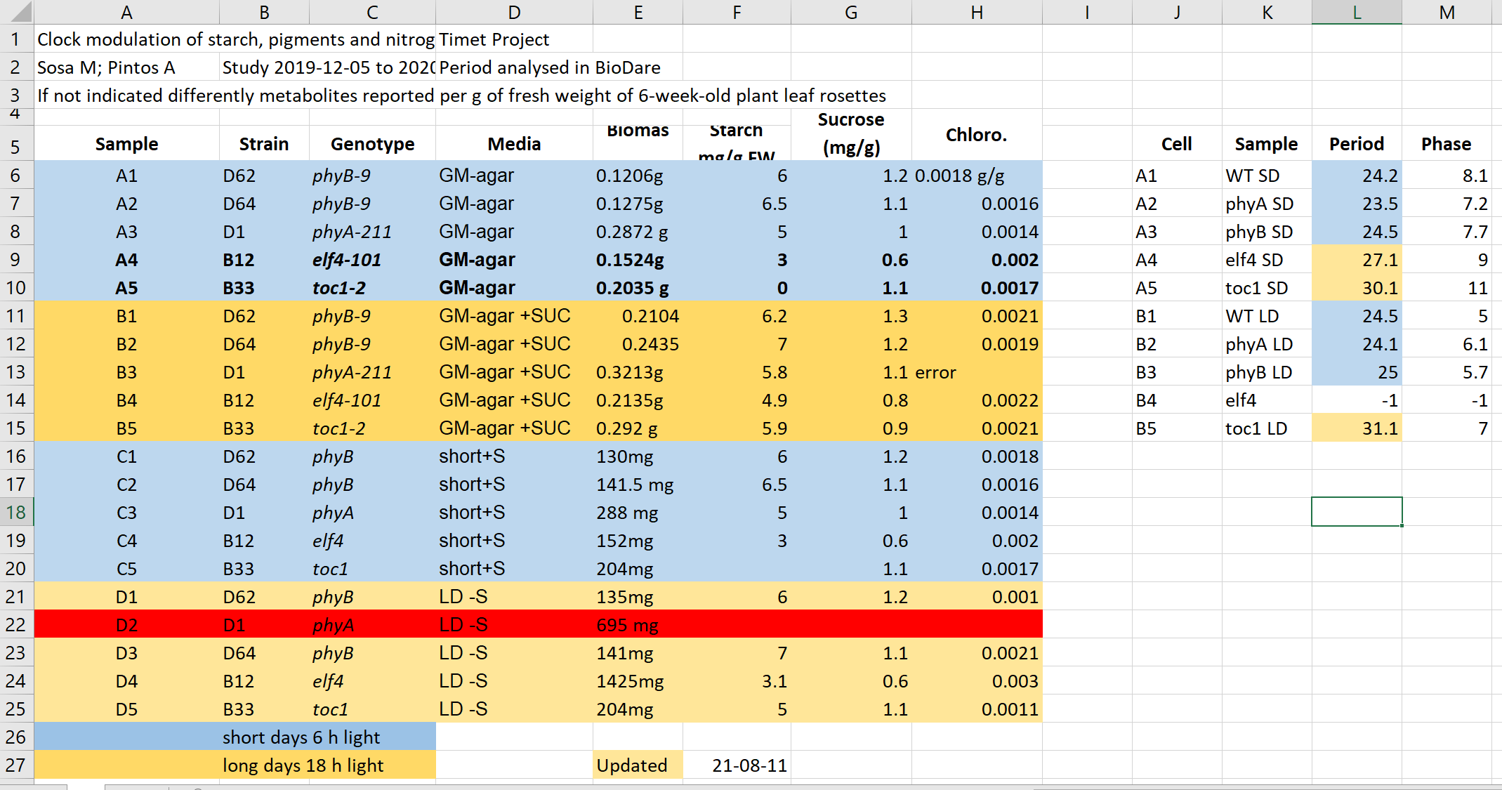
Figure 2
Figure 3
Laboratory records
Figure 1
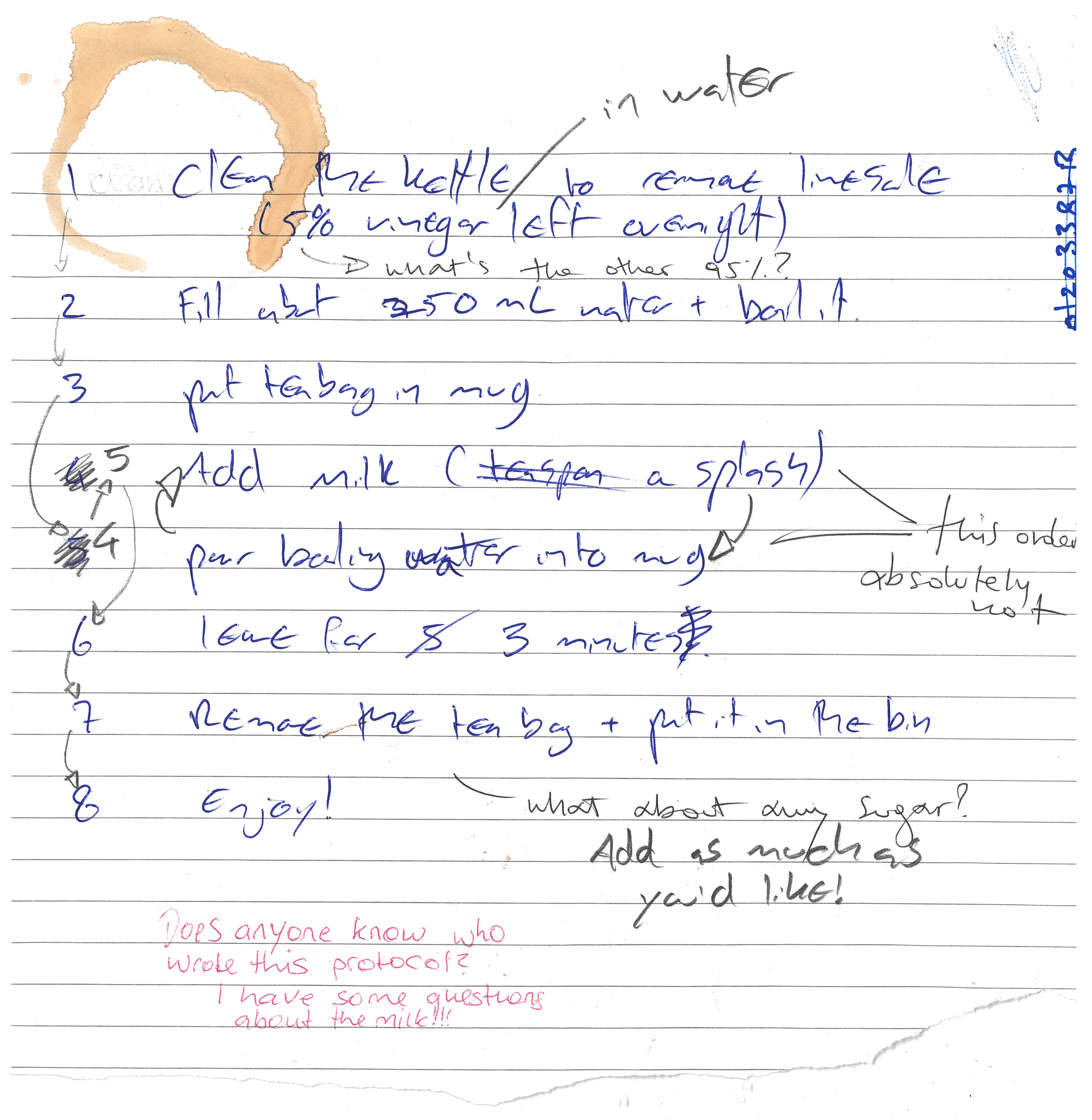
Figure 2
Working with files
Figure 1
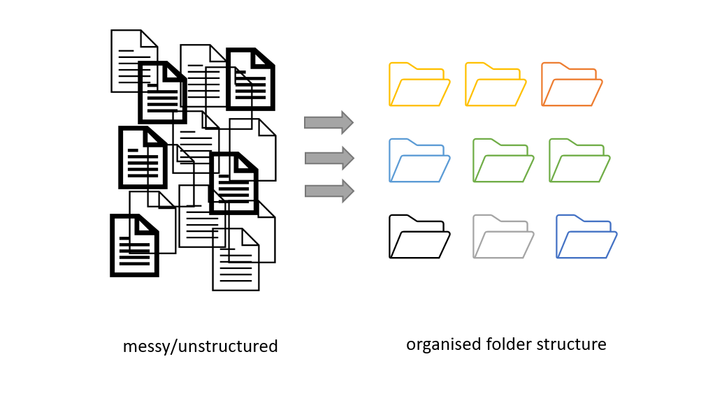 Figure credits: Andrés
Romanowski
Figure credits: Andrés
Romanowski
Figure 2
Have a look at the four different folder structures.
 Figure credits: Ines Boehm
Reusable analysis
Figure 1
Select the notebook titled
‘student_notebook_light_conditions.ipynb’ as depicted below and click
‘Duplicate’. Confirm with Duplicate when you are asked if you are
certain that you want to duplicate the notebook. 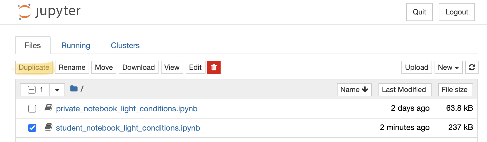 Figure 1. Duplicate a
Jupyter notebook
Figure 1. Duplicate a
Jupyter notebook
Figure 2
A copy of the notebook has appeared with the suffix ‘-Copy’ and a
number (Figure 2a), select this notebook. Have a look
around the notebook and explore its anatomy (Figure 2),
you should see experimental details, an image, and code. If you click on
separate parts of the notebook you can see that it is divided into
individual cells (Figure 2 e-g) which are of varying
type (Code, R in this case, or Markdown - Figure 2d).
Hashtags are comments within the code and shall help you to interpret
what individual bits of code do. 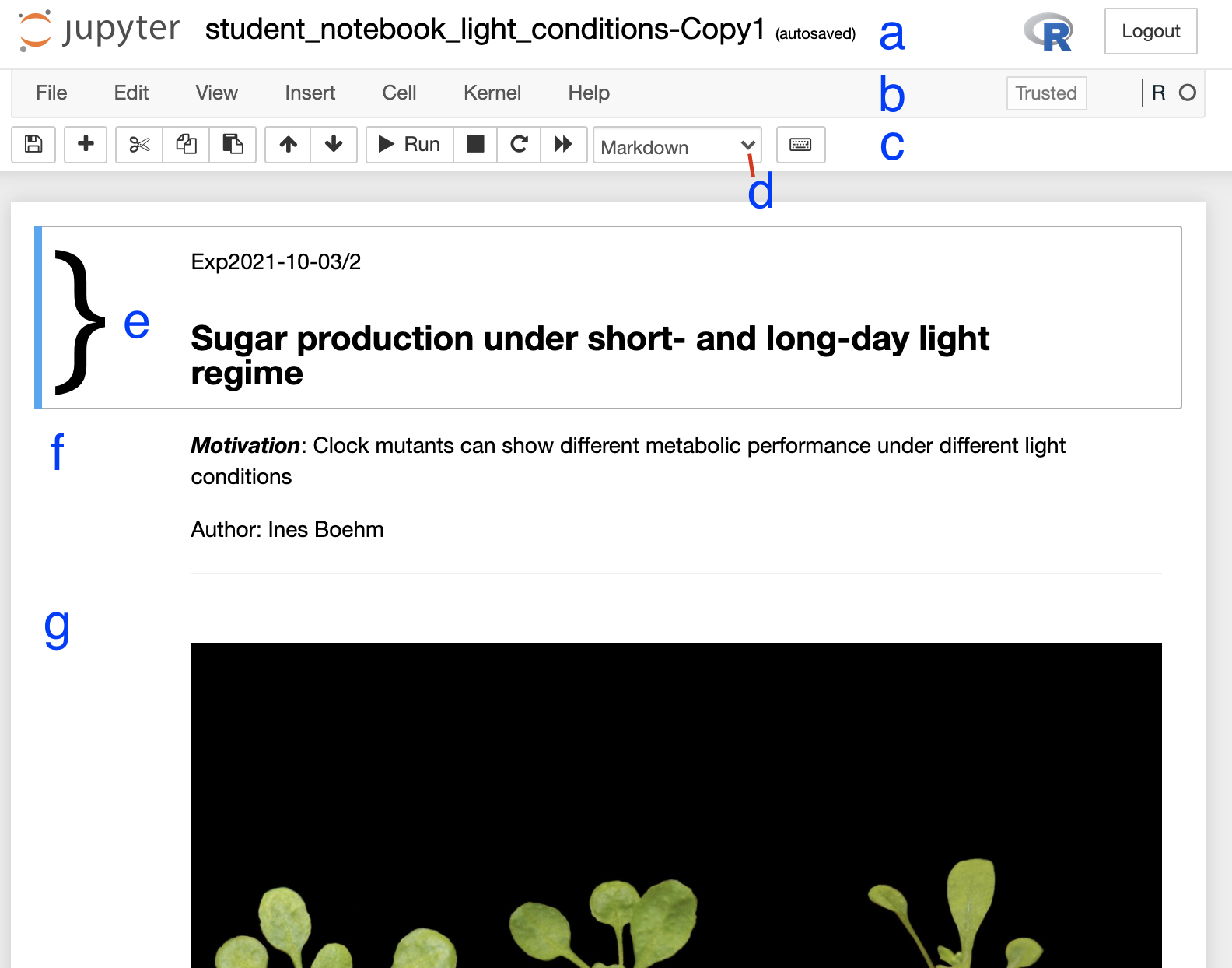 Figure 2. Anatomy of a Jupyter notebook: (a) depicts the name of the
notebook, (b, c) are toolbars, (c) contains the most commonly used
tools, (d) shows of what type - Markdown, Code etc… - the currently
selected cell is, and (e-g) are examples of cells, where (e) shows the
currently selected cell.
Figure 2. Anatomy of a Jupyter notebook: (a) depicts the name of the
notebook, (b, c) are toolbars, (c) contains the most commonly used
tools, (d) shows of what type - Markdown, Code etc… - the currently
selected cell is, and (e-g) are examples of cells, where (e) shows the
currently selected cell.
Figure 3
If you followed all steps correctly you should have reproduced the
table, a graph and statistical testing. Apart from the pre-filled
markdown text the rendered values of the code should look like this:
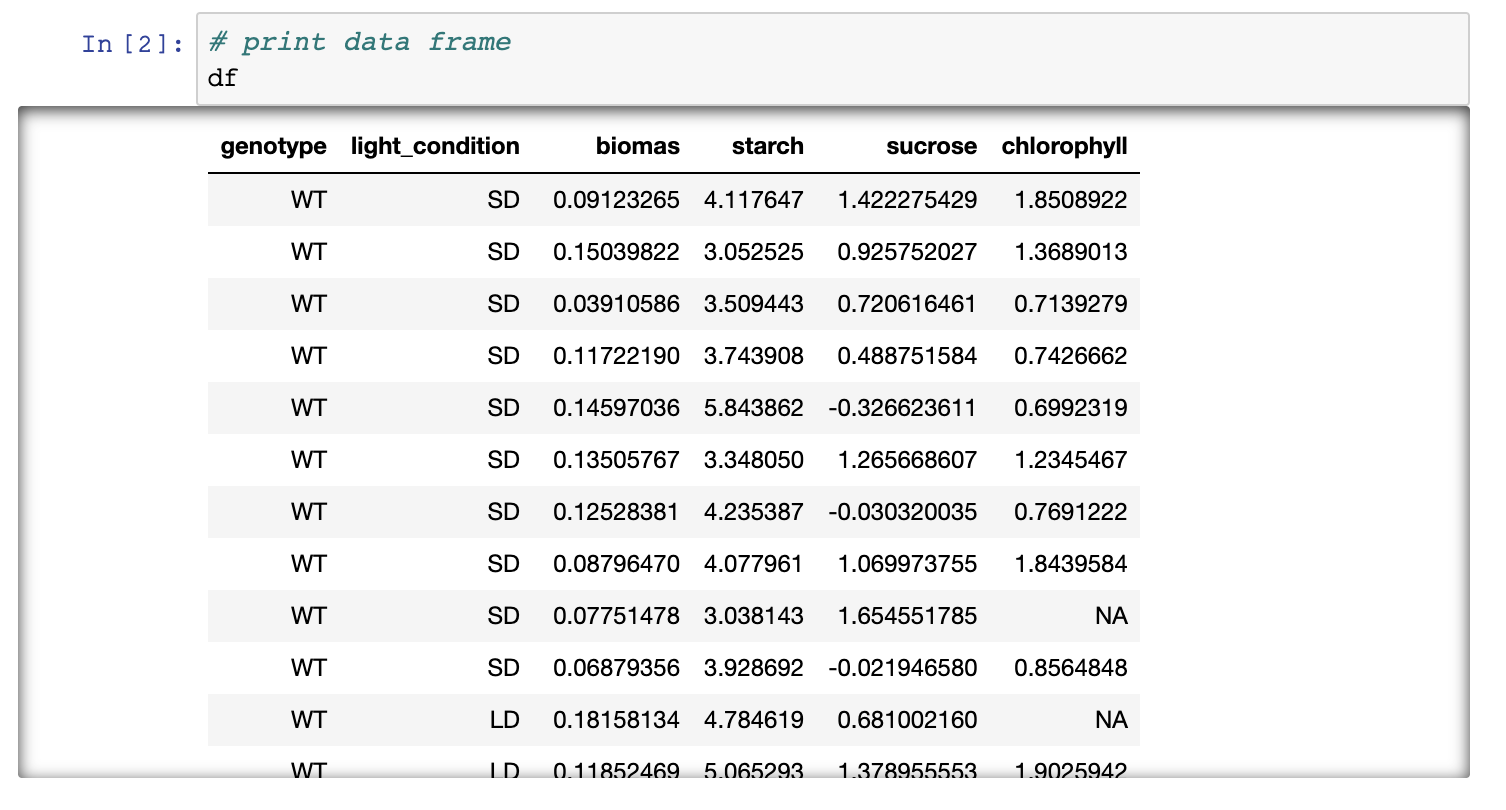 Figure 3. Rendering of
data frame
Figure 3. Rendering of
data frame 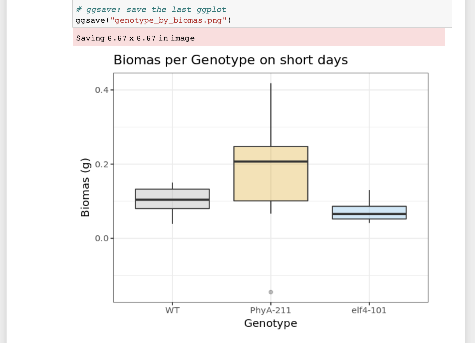 Figure 4. Rendering of
plot
Figure 4. Rendering of
plot
Figure 4
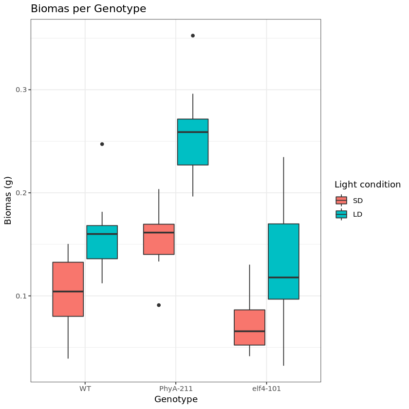 Figure 5. Short- and long-day light
conditions depicted as a grouped boxplot
Figure 5. Short- and long-day light
conditions depicted as a grouped boxplot
Version control
Figure 1

from: Wit and wisdom from Jorge Cham (http://phdcomics.com/)
Figure 2


from: Version control with git (https://carpentries-incubator.github.io/git-novice-branch-pr/01-basics/)
Figure 3
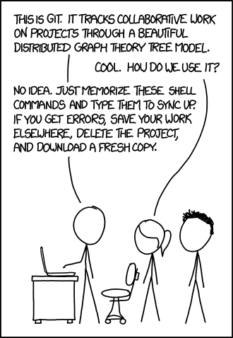
from: xkcd (https://xkcd.com/1597/)
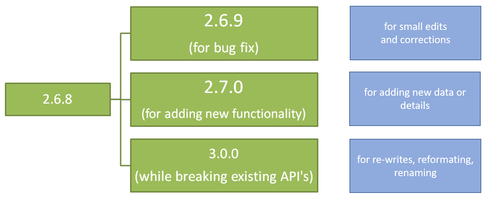
Figure 4
from: Semantic versioning, Parikshit Hooda (https://www.geeksforgeeks.org/introduction-semantic-versioning/)
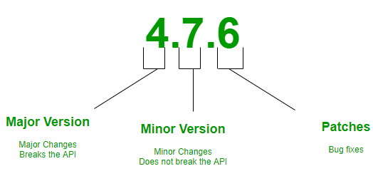
Figure 5
from: Semantic versioning, Parikshit Hooda (https://www.geeksforgeeks.org/introduction-semantic-versioning/)
Templates for consistency
Public repositories
Figure 1
It's all about planning
Figure 1
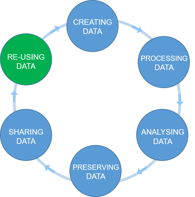 Figure credits:
Tomasz Zieliński
Figure credits:
Tomasz Zieliński
Figure 2
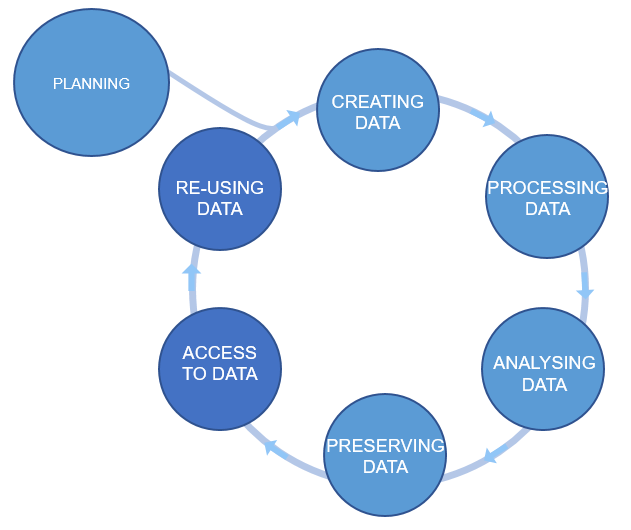 Figure credits: Tomasz Zieliński and Andrés Romanowski
Putting it all together
Template
Figure 1
